You Can't Steer When You Only See the Destination

Why Formulas Show You the Destination, But Charts Show You the Road

1. Endpoints vs. Paths

Every formula in this book tells a CEO where a decision will end. Consider the Sync Tax Multiplier: it shows how many times more expensive each feature becomes as the system grows more interdependent. Then there’s the Total Cost of Complexity, which measures the quarterly bill for an interdependent system. Finally, the Strangler Extraction Cost tells you what you’ll pay to run parallel systems during a modularization.

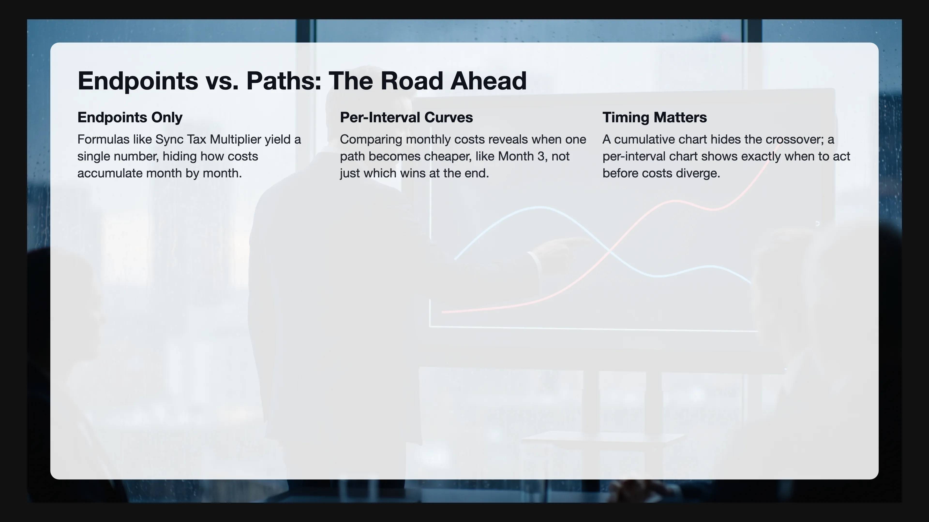
On their own, these are endpoints, single numbers that don’t show how the cost accumulates month by month, or how one curve quietly overtakes another between Month 3 and Month 4.

Without those curves, a CEO who only sees endpoints makes decisions the same way a driver who only sees the destination makes turns. You need the road. You need to know where the curves diverge, where they cross, and which path becomes more expensive before the money is spent.

This article is about building that road. Every chart you’re about to see shows the same fundamental dynamic: two curves of per-interval cost. One curve represents the easy decision, the other the disciplined decision. Time runs along the bottom and cost climbs the side, so the CEO sees not only which path ends higher but exactly when the gap starts to open.

The charts show per-interval cost (monthly or quarterly), not cumulative totals. And this matters because the cumulative total only tells you who won at the end. By comparing per-interval cost, the CEO sees when the curves diverge, and that timing is the information they need. If the modular path becomes cheaper in Month 3, the decision needs to happen before Month 3. A cumulative chart hides that crossover. A per-interval chart puts it in plain view.

Of course, the two curves don’t always represent the same kind of choice. Sometimes the CEO is deciding whether to act, and acting looks expensive but doing nothing compounds the cost (like letting an interdependent system grow without modularizing). Sometimes the CEO is deciding whether to wait, and waiting looks free but acting now prevents a tax that compounds forever (like pushing a feature update during a modularization freeze). At its core, the framework is the same either way: one curve shows the cost of one path, the other shows the cost of the alternative, and the chart reveals which path wins and when.

Today, existing financial visualization tools solve adjacent but different problems. Reinertsen’s Cost of Delay models how deferred value compounds over time (product development flow economics). J-curves from private equity show initial negative returns followed by positive returns. Tornado charts map sensitivity to individual variables. None of these address the specific decision a software CEO faces: comparing the per-interval cost of two architectural paths over time. That gap is where this article lives.

2. Three Curve Patterns

Before walking through the five formulas, it helps to name the shapes you’ll see. Across every chart in this article, three patterns repeat.

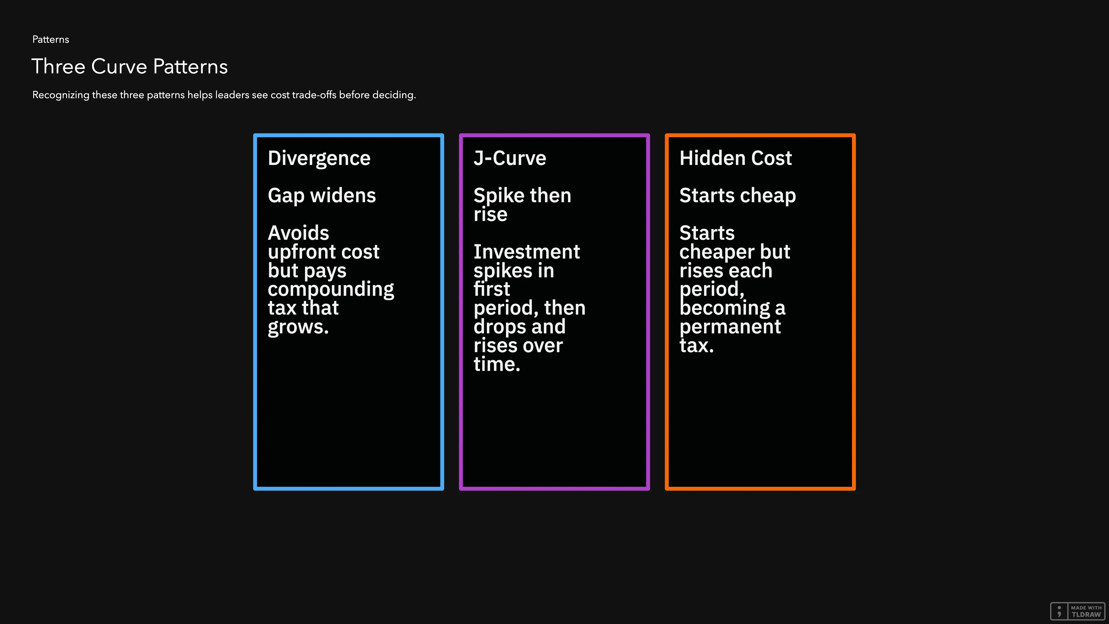
Divergence: one curve bends upward while the other stays flat. The easy choice avoids an upfront cost but pays a compounding tax that grows every month. The disciplined choice pays the upfront cost and eliminates the tax. The gap between the curves widens every single period.

J-Curve: one curve spikes in the first period (the investment), then drops to a low flat line. The other curve starts lower but rises over time. This J-curve is the signature of any investment that pays for itself, and the chart reveals exactly when the payoff happens.

Hidden Cost: one curve starts cheaper, creating the illusion of a saving. But it rises every period, and what looked like a deal becomes a permanent tax. The other curve has a higher starting cost but never compounds.

Most charts in this article show two of these patterns at once. The disciplined path follows a J-curve, while the easy path follows a divergence or a hidden cost. The CEO’s job is to recognize these shapes before the crossover. That recognition is what turns a chart from a visual into a decision.

3. Formula 1: Sync Tax Multiplier

The Sync Tax Multiplier measures how much harder a feature becomes to build as the system grows more interdependent. When $S_t = 1$, a feature takes exactly the effort it should take in a clean system. When $S_t = 3.5$, it takes three and a half times as long because three other modules need updates and two teams need to coordinate. Here, the interdependence is the driver and the multiplier is the result.

The variables:

• $S_t$ = Sync Tax Multiplier (how many times more expensive each feature is compared to a clean system)
• $1$ = the baseline (the work itself, with no extra cost)
• $k$ = Interdependence Factor (how much extra work each dependent module adds, as a fraction of the baseline)
• $C_d$ = Connascence Degree (how many other modules must change when you change one)
• $C_{\text{coord}}$ = Coordination Overhead (hours spent in meetings and reviews that exist only because the system is tangled)
• $E_v$ = Vacuum Effort (the hours a change should take in a perfectly clean system)

$S_t = 1 + k \cdot C_d + \frac{C_{\text{coord}}}{E_v}$

Read it left to right: the baseline ($1$), plus the dependency cost as a fraction of the baseline ($k \cdot C_d$), plus the coordination cost as a fraction of the baseline ($C_{\text{coord}} / E_v$).

The decision: build the next feature inside the interdependent system, or modularize the domain first.

The Monthly Cost Breakdown:

Month	Interdependent System ($S_t$ rising)	Modularize ($S_t = 1$ after extraction)
1	$24,000	$30,000
2	$25,920	$30,000
3	$27,840	$9,600
4	$29,760	$9,600
5	$31,680	$9,600
6	$33,600	$9,600

Assumptions: 2 features per month, vacuum effort $E_v = 40$ hours per feature, blended hourly rate $R$ = $120, interdependence factor $k = 0.5$, connascence degree $C_d$ increases by 0.2 each month as the system gets more tangled. The modularize column includes extraction cost in Months 1 and 2, then drops to the clean-system cost of $E_v \cdot R \cdot 2$ = $9,600 per month.

xychart-beta
    title "Monthly Cost: Build in Interdependent System vs Modularize"
    x-axis [Month 1, Month 2, Month 3, Month 4, Month 5, Month 6]
    y-axis "Cost per Month ($)" 0 --> 35000
    line "Interdependent System (St rising)" [24000, 25920, 27840, 29760, 31680, 33600]
    line "Modularize (St = 1 after extraction)" [30000, 30000, 9600, 9600, 9600, 9600]

What the Non-Tech Leader Sees:

This chart shows a J-curve (the modularize path) crossing a divergence (the interdependent path). Every month, the interdependent system line rises because each new feature makes the system more tangled, so the next feature costs more. In Months 1 and 2, the modularize line spikes because the team is extracting the module, not building features. Then it drops to $9,600 and stays flat forever because new features no longer need coordination with other teams.

By Month 3, the modularize line is already below the interdependent line. By Month 6, the interdependent system costs $24,000 more in that month alone. Best of all, the extraction paid for itself in two months, and everything after is profit.

4. Formula 2: Total Cost of Complexity

The Total Cost of Complexity is the full price of operating an interdependent system for one period. In a single figure, it adds up the cost of hidden dependencies, the cost of human coordination, and the cost of maintenance and infrastructure that a clean system would not need, then multiplies by the risk of regressions (changes that break unrelated features).

The variables:

• $T\mathbb{C}$ = Total Cost of Complexity (the full dollar cost of running a tangled system for one period)
• $CDC$ = Connascence Degree Cost (the dollar cost of hidden dependencies between modules)
• $STC$ = Sync-Tax Cost (the dollar cost of coordination overhead: meetings, reviews, and threads that exist only because the system is tangled)
• $E\mathbb{C}$ = Excess Complexity Cost (maintenance and infrastructure that exist only because the system is tangled, not because customers asked for new things)
• $R_m$ = Failure Risk Multiplier (how much regressions inflate the true cost, from Formula 3 below)

$T\mathbb{C} = ((CDC + STC) + E\mathbb{C}) \cdot R_m$

Read it left to right: add the cost of hidden dependencies ($CDC$) and the cost of coordination ($STC$), add the cost of excess maintenance and infrastructure ($E\mathbb{C}$), then multiply by the risk that something breaks ($R_m$).

The decision: keep building in the interdependent system, or modularize at the efficiency threshold.

The Quarterly Cost Breakdown:

Quarter	Interdependent Trajectory	Modular Trajectory
Q1	$125,000	$75,000
Q2	$185,000	$78,000
Q3	$265,000	$80,000
Q4	$380,000	$82,000

Assumptions: 20 features per quarter, vacuum effort $E_v = 40$ hours per feature, blended hourly rate R = $120, interdependence factor $k = 0.5$. In the interdependent trajectory, connascence degree $C_d$ and regression rate $R_t$ both increase each quarter, driving $T\mathbb{C}$ upward. In the modular trajectory, $C_d$ stays bounded and $R_t$ stays near zero, so cost grows only with genuine feature volume.

xychart-beta
    title "Quarterly Cost: Interdependent System Trajectory vs Modular Trajectory"
    x-axis [Q1, Q2, Q3, Q4]
    y-axis "Cost per Quarter ($)" 0 --> 400000
    line "Interdependent (Cd and Rt growing)" [125000, 185000, 265000, 380000]
    line "Modular (bounded)" [75000, 78000, 80000, 82000]

What the Non-Tech Leader Sees:

This chart is a pure divergence. Each quarter, the interdependent trajectory accelerates because the system gets more fragile and more tangled. Q4 costs three times what Q1 cost. In contrast, the modular trajectory rises only by $2,000 per quarter, which is just the cost of building more features. There is no acceleration because there is no tax on complexity.

By Q4, the interdependent system costs $298,000 more in a single quarter. That’s a full engineering team.

5. Formula 3: Failure Risk Multiplier

The Failure Risk Multiplier measures how much regressions (changes that break unrelated features) inflate the true cost of a change. When $R_m = 1.2$, the true cost is 20% above the build estimate. When $R_m = 2.6$, the true cost is 160% above the estimate because every change has a high probability of breaking something else.

The variables:

• $R_m$ = Failure Risk Multiplier (how much the true cost exceeds the build estimate)
• $1$ = the base cost with zero risk
• $R_t$ = Regression Rate (how often a change breaks something unrelated, measured as regressions divided by total changes)
• $C_f$ = Incident Cost (the dollar cost of a single regression: engineering time to fix it plus business impact like downtime and lost revenue)
• $\mathbb{C}$ = Cost of Complexity (the base cost of the change before risk adjustment)

$R_m = 1 + \frac{R_t \times C_f}{\mathbb{C}}$

Read it left to right: start with the base cost ($1$), then add the expected failure cost ($R_t \times C_f$) as a fraction of the base cost ($\mathbb{C}$). When nothing ever breaks ($R_t = 0$), the multiplier is 1 and the cost is just the cost. When regressions are frequent and expensive, the multiplier inflates the total proportionally.

The decision: ship features now with the current regression rate, or invest in reducing $R_t$ first.

The Monthly Cost Breakdown:

Month	Ship Now ($R_t$ growing, $R_m$ rising)	Reduce $R_t$ First ($R_m = 1.2$)
1	$32,000	$25,000
2	$36,000	$24,000
3	$40,000	$24,000
4	$44,000	$24,000
5	$48,000	$24,000
6	$52,000	$24,000

Assumptions: 2 features per month, base cost per feature $\mathbb{C}$ = $10,000, incident cost $C_f$ = $40,000. In the “ship now” path, regression rate $R_t$ grows by 0.05 each month as the system gets more fragile, driving $R_m$ upward. In the “reduce first” path, the team invests $25,000 in Month 1 to bring $R_t$ down, then ships with $R_m = 1.2$ (a 20% risk premium).

xychart-beta
    title "Monthly Cost: Ship with Growing Risk vs Reduce Regression Rate First"
    x-axis [Month 1, Month 2, Month 3, Month 4, Month 5, Month 6]
    y-axis "Cost per Month ($)" 0 --> 55000
    line "Ship now (Rt grows, Rm rises)" [32000, 36000, 40000, 44000, 48000, 52000]
    line "Reduce Rt first (then Rm = 1.2)" [25000, 24000, 24000, 24000, 24000, 24000]

What the Non-Tech Leader Sees:

This chart shows a J-curve crossing a divergence. Every month, the “ship now” line rises by $4,000 because each feature ships into a more fragile system, so the next feature is more likely to break something. The risk premium compounds. On the other side, the “reduce first” line has a $25,000 investment in Month 1, then stabilizes at $24,000 because regressions are rare.

By Month 6, shipping now costs $28,000 more in that month. The gap widens by $4,000 every month forever.

6. Formula 4: Strangler Extraction Cost

The Strangler Extraction Cost measures the cost of running old and new systems in parallel during a modularization. A strangler extraction is a gradual replacement where a new, clean module grows around the old system until the old system can be removed. When leadership respects the change freeze, the sync layer (the code that keeps old and new systems aligned) is simple and the extraction finishes on schedule. When leadership violates the freeze, the sync layer must handle divergent data, and the cost explodes.

The variables:

• $C_{total}$ = total cost of the extraction
• $ETC$ = Extraction Team Cost per month (the team building the new module)
• $T$ = duration in months (how long old and new systems run in parallel)
• $C_{sync}$ = sync layer cost per month (the team keeping old and new systems aligned, assuming the data copy is trivial)
• $S_t$ = Sync Tax Multiplier (how coupled the sync layer is to the rest of the system, from Formula 1 above)
• $\mathbb{M}$ = Magnitude Multiplier (how complex the data transformation between old and new systems is, where 1 means a simple copy and 4 means heavy translation)

$C_{total} = (ETC \times T) + (C_{sync} \times T \times S_t \times \mathbb{M})$

Read it left to right: the build cost ($ETC \times T$) plus the sync cost, where the sync cost compounds through duration ($T$), coupling ($S_t$), and transform complexity ($\mathbb{M}$). Double any one of those and the sync cost doubles. When all three increase at the same time, which is what happens when leadership allows product changes during extraction, the cost grows exponentially.

The decision: respect the change freeze during extraction, or allow product changes to continue.

The Monthly Cost Breakdown:

Month	Violate Freeze	Respect Freeze
1	$96,000	$96,000
2	$110,400	$96,000
3	$136,500	$96,000
4	$168,000	$96,000
5	$218,400	$96,000
6	$294,900	$96,000
7	$480,000	$15,000
8	$480,000	$15,000
9	$480,000	$15,000
10	$480,000	$15,000
11	$480,000	$15,000
12	$480,000	$15,000

Assumptions: extraction team cost ETC = $60K per month, sync layer cost $C_{sync}$ = $30K per month. Under the respect-freeze path, extraction completes in 6 months ($T = 6$) with low coupling ($S_t = 1.2$) and simple data copy ($\mathbb{M} = 1$), then the sync layer dies and monthly cost drops to $15,000. Under the violate-freeze path, each product change forces the sync layer to handle divergent data, $\mathbb{M}$ climbs from 1 to 4, $S_t$ rises, and $T$ extends to 24 months.

xychart-beta
    title "Monthly Cost: Violate Freeze vs Respect Freeze (12 Months)"
    x-axis [M1, M2, M3, M4, M5, M6, M7, M8, M9, M10, M11, M12]
    y-axis "Cost per Month ($)" 0 --> 500000
    line "Violate freeze (M and St exploding)" [96000, 110400, 136500, 168000, 218400, 294900, 480000, 480000, 480000, 480000, 480000, 480000]
    line "Respect freeze (6mo then clean)" [96000, 96000, 96000, 96000, 96000, 96000, 15000, 15000, 15000, 15000, 15000, 15000]

What the Non-Tech Leader Sees:

This chart shows a divergence that turns into a cliff. The “violate” line bends upward because one product change forces the sync layer to handle two divergent data models. The transformation complexity grows. By Month 7, the extraction is still not done and the monthly cost hits $480,000. On the other side, the “respect” line stays flat at $96,000 for 6 months, then drops to $15,000 when the sync layer dies and the old system is removed.

The CEO sees that one feature request doesn’t cost $50,000. It costs $50,000 plus $384,000 per month in extended sync maintenance.

7. Formula 5: Connascence Cost

The Connascence Cost measures the tax paid when modules share hidden dependencies. Connascence is a measure of coupling: two modules are connascent when a change in one forces a change in the other. When $C_d = 3$, three modules must change together, and every feature pays $3,600 extra. When $C_d = 0$, modules evolve independently.

The variables:

• $CDC$ = Connascence Degree Cost (the dollar cost of hidden dependencies between modules)
• $C_d$ = Connascence Degree (how many other modules must change when you change one)
• $k$ = Interdependence Factor (how much extra work each dependent module adds, as a fraction of the baseline)
• $E_v$ = Vacuum Effort (the hours a change should take in a perfectly clean system)
• $R$ = blended hourly rate (developer, QA, ops, all in)

$CDC = C_d \cdot k \cdot E_v \cdot R$

Read it left to right: count the connascent modules ($C_d$), multiply by the average extra effort per module ($k \cdot E_v$), and convert to dollars ($R$).

The decision: accept a convenient coupling for speed, or design a clean interface that costs more today but eliminates the tax.

The Monthly Cost Breakdown:

Month	Accept Coupling ($C_d$ growing)	Clean Interface ($C_d = 0$)
1	$14,400	$15,000
2	$16,800	$9,600
3	$16,800	$9,600
4	$19,200	$9,600
5	$19,200	$9,600
6	$21,600	$9,600

Assumptions: 2 features per month, vacuum effort $E_v = 20$ hours per feature, blended hourly rate $R$ = $120, interdependence factor $k = 0.5$. In the “accept coupling” path, connascence degree $C_d$ grows from 2 to 5 as more modules become entangled. In the “clean interface” path, the team invests $15,000 in Month 1 to design a clean interface, then $C_d = 0$ and each feature costs only the baseline $E_v \cdot R \cdot 2$ = $9,600.

xychart-beta
    title "Monthly Cost: Accept Coupling vs Design Clean Interface"
    x-axis [Month 1, Month 2, Month 3, Month 4, Month 5, Month 6]
    y-axis "Cost per Month ($)" 0 --> 25000
    line "Accept coupling (Cd grows)" [14400, 16800, 16800, 19200, 19200, 21600]
    line "Clean interface (then Cd = 0)" [15000, 9600, 9600, 9600, 9600, 9600]

What the Non-Tech Leader Sees:

This chart shows a hidden cost crossing a J-curve. The “accept coupling” line rises as more modules become entangled, and a change in one module now breaks three others. For the “clean interface” line, a $15,000 design cost appears in Month 1, then drops to $9,600 and stays flat because no other modules need to change.

By Month 2, the clean interface is already cheaper. By Month 6, the coupling choice costs $12,000 more in that month. The “one-time convenience” has become a permanent tax.

8. What Every Chart Shows

Every chart in this article follows the same pattern:

• Time on the horizontal axis.
• Cost on the vertical axis.
• Two curves: the easy decision and the disciplined decision.
• Per-interval cost, not cumulative totals.

The value is not in the final numbers. The value is in the shape. When a CEO sees a line that bends upward, they know the system is compounding waste. And when a CEO sees a line that spikes then goes flat, they know the investment has a payoff. When two lines cross at Month 3, the CEO knows the decision must be made before Month 3.

Without the curves, every decision is a bet on a single number. With the curves, the decision is an informed choice between two trajectories.

9. Conclusion

The formulas in this book are not abstractions. They’re economic models. But a model that produces a single number hides the most important question: when does the cost start to diverge?

A CEO who only sees the endpoint of the Sync Tax Multiplier might approve a feature that looks profitable. But a CEO who sees the two curves knows the profit evaporates between Month 3 and Month 4. Similarly, a CEO who only sees the endpoint of the Strangler Extraction Cost might approve one product change during extraction. In contrast, a CEO who sees the two curves knows that one change turns a $96,000 monthly cost into a $480,000 monthly cost.

The curve is the truth, and the endpoint is just the summary. And summaries, by definition, leave out the story.

The standard is simple. Every architectural decision presented to the CEO must include two curves, because the only way to choose the right path is to see both at the same time.

References

• Cost of Delay. Don Reinertsen, The Principles of Product Development Flow: Second Generation Lean Product Development (Celeritas Publishing, 2009). Wikipedia summarizing Reinertsen’s concept of quantifying the economic impact of delayed product delivery.
• J-Curve (Private Equity) — The standard descriptive model for private equity fund returns, where initial negative returns from fees and early investments are followed by positive realized gains. Investopedia, Moonfare.
• Tornado Chart — A horizontal bar chart for one-way sensitivity analysis, used in financial modeling to rank variables by impact on output metrics like NPV or IRR. Corporate Finance Institute.

Measure it

Read the cost curve before you fund the endpoint

The Sync Tax multiplier shows where a decision ends, and the curve shows the cost compounding while attention stays on that endpoint. The calculator returns the multiplier behind the curve for one change.

• Measure the multiplier behind this curve →
• See this cost curve in Defusor →