The Setup That Turns a 20-Hour Feature Into an 80-Hour One

Quantifying the Invisible Friction

Efficiency is not a feel-good word. Think of it as a ratio: the value the product produces for the customer divided by the total effort the company spends to produce it. Making that ratio visible and showing what pulls it down is this article’s job.

In any product company past product-market fit, the single biggest weight on the ratio is the Sync Tax: the extra effort a change has to spend because the system is too interdependent for its size and market share. Think of the Sync Tax as a multiplier on the real work. A feature that should take 20 hours can easily take 80, and the difference is the setup they have to work inside. That setup includes the code, the way it’s wired together, the teams it crosses, the meetings, the reviews, and the contracts between groups. Because of that setup, the change costs four times more than it should.

Beyond the definition, the rest of this article builds the math to make that multiplier undeniable for a CEO, and shows how to use it to forecast cost, track structural health, and trigger decisions before the system freezes.

1. Defining the Sync Tax Multiplier

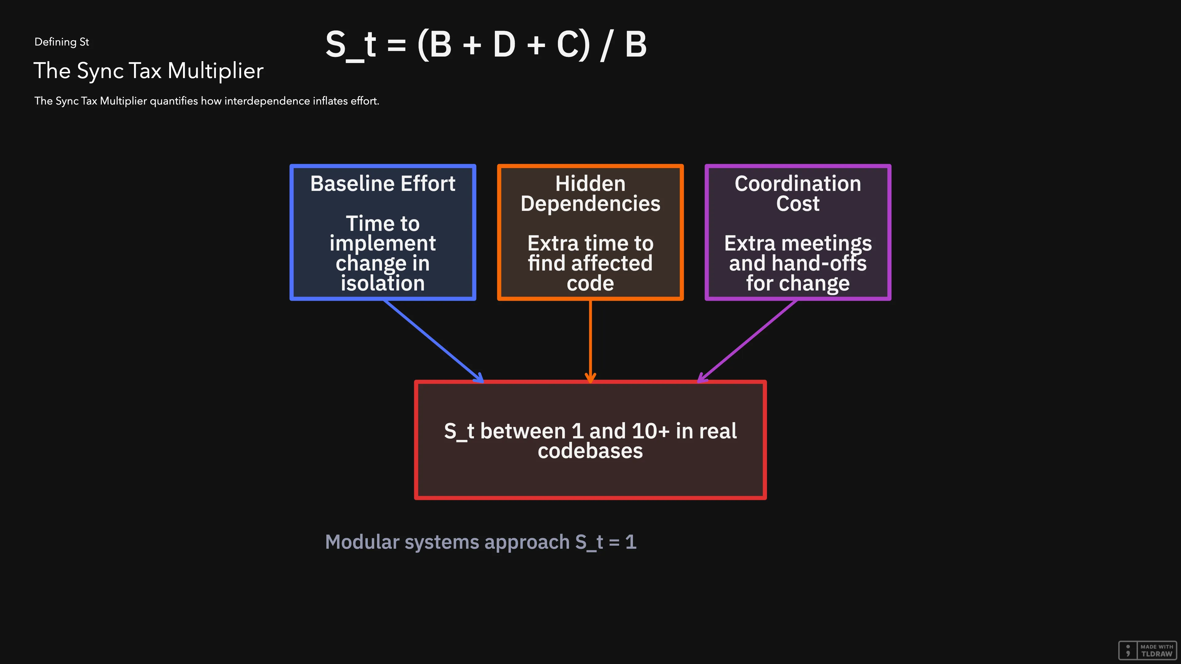
The Sync Tax Multiplier, written as $S_t$, is a single number that captures the compounding effect of all the extra work caused by interdependence. In codebases past product-market fit that have never been modularized, $S_t$ sits between 2 and 6. In ones that have grown tangled for years, it can climb past 10. A modular system has $S_t$ close to 1, meaning every change costs roughly what it should. The rest of this section defines the three components that make up the multiplier, then assembles them.

The baseline, $E_v$: what the work should cost

Before measuring how bad the cost is today, the formula needs a baseline: how much would this change cost if the system were perfectly modular, with no hidden dependencies and no coordination overhead? That baseline is called the Vacuum Effort, written as $E_v$.

Imagine a developer needs to add a new field to a customer profile. In a perfectly modular system, the change touches one file, one test, one deployment, and that is $E_v$: the time the change should take, measured in hours. The Sync Tax measures how far reality has drifted from $E_v$.

To turn the time into money, multiply by $R$, the loaded hourly rate of the engineering team. “Loaded” means the estimated full cost of an engineer to the company: salary, benefits, equipment, management overhead, all of it. The dollar version of the baseline is $E_v \cdot R$.

Hidden dependencies: the cost of forced changes

The term for that kind of forced coupling is connascence, coined by Meilir Page-Jones in the 1990s and adopted by Ford, Parsons, and Kua in Building Evolutionary Architectures. Two components are connascent when a change in one forces a change in the other. For the metric of efficiency, all that matters is the count.

The Connascence Degree, written as $C_d$, is the count of unrelated modules that have to change together with the main one for a given change. A high $C_d$ shows that a single change is forcing many others to move with it.

But not every connascent module adds the same amount of work. Some are tightly coupled and require extensive rework; others need only a small adjustment. The Interdependence Factor, written as $k$, captures the average share of extra effort that each extra module adds. Calibrate $k$ from past tasks by dividing the total extra module effort by $C_d \cdot E_v$. Until a company has done that calibration, $k = 0.5$ is a reasonable starting point: each connascent module adds roughly half the baseline effort in extra work. It is not a measurement, and the resulting $S_t$ will be approximate, but the magnitude is what matters for the trade-off the multiplier is designed to show.

Read $C_d$ as the number of forced companions, and $k \cdot E_v$ as the average extra work per companion. The dollar cost of hidden dependencies is the count times the average extra work per module, all converted to dollars. In math, that’s $C_d \cdot k \cdot E_v \cdot R$, read left to right: count the connascent modules ($C_d$), multiply by the average extra effort per module ($k \cdot E_v$), and convert to money ($R$). Article 5 gives this dollar component a name, the Connascence Degree Cost $CDC$, and uses it inside the Total Cost of Complexity formula.

Coordination overhead: the cost of forced conversations

Hidden technical dependencies are not the only cost. Tangled systems also force people to coordinate. Adding that new customer field might require a meeting with the billing team, a Slack thread with the search team, and a code review with someone who built the original schema years ago. None of that is in the code but in the calendar.

The Coordination Overhead, written as $C_{\text{coord}}$, is the total number of hours the team spends in meetings, threads, calls, and reviews that exist only because the system is tangled. In a modular system, those hours would not be needed to be spent.

The dollar cost of coordination is the hours times the loaded rate, or $C_{\text{coord}} \cdot R$ in math. Article 5 gives this dollar component a name, the Sync-Tax Cost $STC$, and uses it inside the Total Cost of Complexity formula.

Assembling the multiplier, $S_t$: a ratio of three costs

Now the three components are in place: the baseline ($E_v \cdot R$), the hidden-dependency cost ($C_d \cdot k \cdot E_v \cdot R$), and the coordination cost ($C_{\text{coord}} \cdot R$). The multiplier $S_t$ is the ratio of the all-in cost to the baseline. Written as a formula:

$S_t = 1 + k \cdot C_d + \frac{C_{\text{coord}}}{E_v}$

Read it left to right:

• $1$ is the baseline, the work that should happen.
• $k \cdot C_d$ is the dependency cost expressed as a fraction of the baseline: $C_d$ modules each adding $k$ times the baseline effort.
• $C_{\text{coord}} / E_v$ is the coordination cost expressed as a fraction of the baseline work.

When $S_t = 1$, the system is clean, and every change costs what it should. When $S_t = 3$, the company is paying three times the baseline cost of change, and that ratio applies to every feature, every quarter, until something changes.

This is the simplest form of the formula. In practice, different connascent modules add different amounts of work, so the most general form sums a per-module effort $e_i$ across all $C_d$ modules. The simplified form above assumes every module adds the same average share, captured by $k$. For day-to-day use, the simplified form is enough. The general form is a footnote, not a tool.

The dollar cost: turning the multiplier into money

$S_t$ translates directly into a cost multiplier once the loaded hourly rate $R$ is applied to the baseline:

Total Project Cost $= (E_v \cdot R) \cdot S_t$

The extra cost caused by the Sync Tax is the baseline cost multiplied by $(S_t - 1)$:

$(E_v \cdot R) \cdot (S_t - 1)$

This framing makes the Sync Tax tangible for business stakeholders: every full unit added to $S_t$ costs the company $E_v \cdot R$ dollars on that change alone, and the same multiplier applies to every future change.

A worked example

A feature that would take 20 hours in a clean system has to update three unrelated modules and triggers 10 hours of meetings, threads, and reviews.

• $E_v = 20$ hours (the baseline)
• $C_d = 3$ (three other modules have to change)
• $k = 0.5$ (each extra module adds 50% of $E_v$. Used here as a teaching assumption; real values vary)
• $C_{\text{coord}} = 10$ hours (coordination overhead)

Plug into the multiplier:

$S_t = 1 + 0.5 \cdot 3 + \frac{10}{20} = 1 + 1.5 + 0.5 = 3.0$

The total effort for the feature is $E = 20 \times 3.0 = 60$ hours, a 300% tax over the baseline. With $R$ = $120 per hour:

• Cost without Sync Tax: 20 hours × $120 = $2,400
• Cost with Sync Tax: 60 hours × $120 = $7,200
• Extra monetary cost: $7,200 − $2,400 = $4,800 (a 300% increase, matching the time multiplier)

A more visceral example

Picture a feature for “tiered pricing support.” The real work of writing the pricing logic is 20 hours. But the change has to touch the User, Billing, Search, and Checkout modules just to add a pricing field, plus four more modules that share dependencies with them. $C_d$ is high: eight modules have to be updated together. The total effort becomes 80 hours. The CEO isn’t paying for the pricing field. The company is paying a 60-hour tax to make sure Spanish doesn’t break shipping labels in some unrelated part of the system.

Gathering the inputs: a forcing function, not a measurement

These inputs are not measured the way revenue or headcount is. They require inference, calibration, and judgment, and a company will not have clean data for them on day one. The metric is designed to force the conversation that produces the data, not to wait for the data to appear. A rough $S_t$ is more useful than no $S_t$ at all. Each company will track different things, and the right level of rigor depends on the size of the decision the metric is being used to inform.

$E_v$ is the easiest input to get. It is an expert estimate of how long the change would take in a perfectly clean system, with no hidden dependencies and no coordination overhead. The company has never built a clean version, so the estimate is itself a guess, but it is a guess any senior engineer can make. The CEO asks the engineering lead: “If we threw away everything we have and built this from scratch, how long would it take?” The answer is $E_v$.

$C_d$ is partially automatable, but only inside a single repository. In a monorepo, git log --stat and dependency-graph tools can count the number of files or modules a change touches. In a multi-repository architecture, the relevant dependencies live in different repositories with no shared history, so no single tool sees the full picture. The count of “unrelated” modules is also a judgment call: was that module related or coincidental? The CEO asks the engineering lead: “When we ship a feature, how many other modules typically have to change with it?” A number like “between 3 and 6” is enough to compute the multiplier.

$k$ is for calibration, not measurement. The formula is $k$ = (total extra module effort) / $(C_d \cdot E_v)$, and it requires data the company does not have on day one. The honest path is to pick one real project, estimate $E_v$ and $C_d$, measure the actual effort, and compute $k$ once. The result becomes the de facto value for the company until something changes. In tightly coupled systems, $k$ often is above 1.0. In loosely coupled systems, it can be 0.2 or lower. Until a company has done the calibration, $k = 0.5$ is a reasonable starting point. The multiplier computed with a guessed $k$ will be approximate, but the magnitude is what matters for the trade-off the metric is designed to show.

$C_{\text{coord}}$ is the most fragmentary. Calendar logs, Slack history, and code review times are not tracked as a single line item, so the number has to be reconstructed. The CEO asks the engineering lead: “How much of last quarter’s engineering time went into meetings, threads, and reviews that existed only because the system is tangled?” The answer is an estimate, and that’s fine. The metric is a forcing function: the act of asking is what makes the team notice.

The first time the CEO asks for these numbers, the engineering team will not have them. That absence is the point. The metric exists to make the lack of data visible, so the team has a reason to start tracking it. After two or three cycles, the inputs become data. Until then, rough estimates are enough to compute a rough $S_t$, and a rough $S_t$ is enough to make the trade-off visible.

2. Forecasting the Cost of Complexity

The Sync Tax Multiplier lets leaders forecast the future cost of complexity under different architectural choices. Article 5’s Total Cost of Complexity (TCC) formula ties the multiplier to the all-in dollar cost: the cost of hidden dependencies ($CDC$), the cost of coordination ($STC$), the maintenance and infrastructure overhead, all multiplied by the failure risk multiplier. The full derivation lives in Article 5.

Each component grows differently depending on the architecture:

• Interdependent trajectory:
  • $C_d(t)$ increases as features accumulate, raising the connascence-degree cost and the coordination cost.
  • The regression rate $R_t(t)$ grows as the system becomes more fragile, lifting the failure risk multiplier $R_m(t)$.
  • Maintenance and infrastructure overhead $M(t) + I_c(t)$ expand because patches, migrations, and sync jobs compound every quarter.
• Modular trajectory:
  • $C_d(t)$ stays bounded because changes are isolated to one module.
  • $R_t(t)$ stays near zero, keeping $R_m(t) \approx 1$.
  • $M(t) + I_c(t)$ grows only with genuine business-logic expansion, not with accidental complexity.

A 12-month projection

Assume a team delivers 20 features per year. In an interdependent system, each new feature increases the average Connascence Degree by 0.2 modules and the Regression Rate by 0.01. Using the formulas from Article 5, the projected TCC for each quarter looks like this:

Quarter	$C_d$	$R_t$	$S_t$	$T\mathbb{C}$ (interdependent)	$T\mathbb{C}$ (modular)
Q1	2.0	0.05	2.5	$125k	$75k
Q2	2.4	0.08	3.1	$185k	$78k
Q3	2.8	0.12	3.8	$265k	$80k
Q4	3.2	0.17	4.6	$380k	$82k

Assumptions: $E_v = 40$ h/feature, $R$ = $120/h, $k = 0.5$ (teaching value, not a recommendation), baseline $M + I_c$ = $50k/quarter.

Plain-English read: in the interdependent column, the cost roughly triples over a year because each new feature forces more modules into the change and the risk of breaking something else climbs with every release. In the modular column, the cost rises only with genuine business growth, the same kind of growth that pays for itself.

Where this leads

The same dynamic, played out over years, is what makes a system feel like it has slowed down. A change that took 120 hours a few years ago can easily take 600 hours today, and the Sync Tax Multiplier has gone from 1.2 to 6.0 in the meantime. The system is now absorbing 80% of every dollar spent on engineering before any of it reaches the customer. That trajectory is the warning sign the metric is designed to show.

3. Counting the Friction: The Structural Metrics

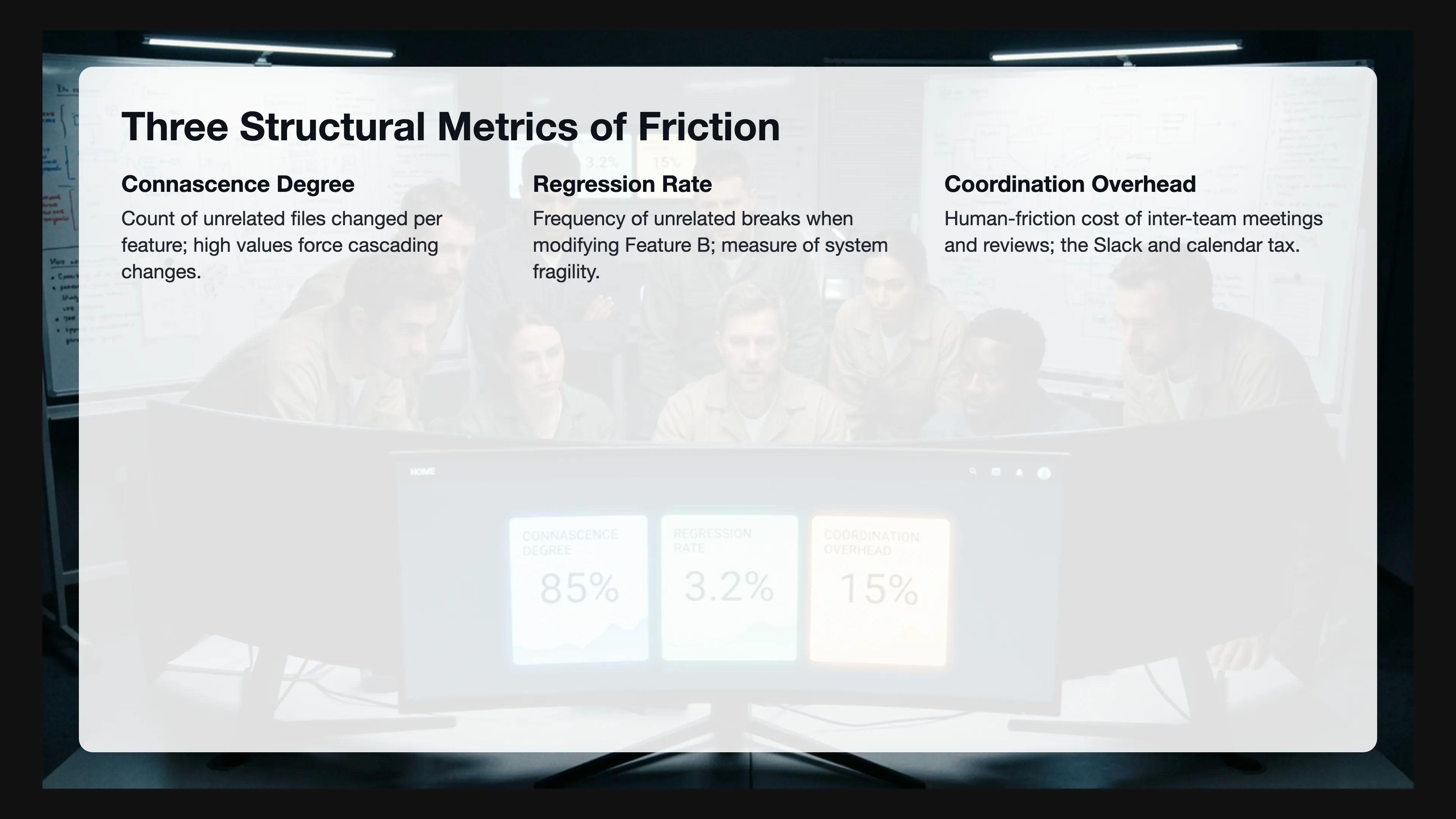
To move away from gut-feeling estimates, the CEO holds the engineering team accountable for providing automated, data-driven metrics that explain the state of the multiplier. Each metric answers one specific question.

• Connascence Degree ($C_d$): the count of unrelated files or modules that have to be modified to implement a single feature. A high $C_d$ shows that a single change is forcing many others to move with it. When components share a connascence relationship, changing one forces changes in the others, and $C_d$ is the count of those forced companions.

• Degree of Interdependence (Fan-Out): the count of foreign database relations or external modules that a specific component touches. It is the inbound and outbound dependency count of a single module.

• Regression Rate ($R_t$): the frequency of “unrelated breaks,” meaning bugs appearing in Feature A when Feature B is modified. $R_t$ is the measure of system fragility, and it feeds directly into the Failure Risk Multiplier $R_m$ in Article 5.

• Coordination Overhead ($C_{\text{coord}}$): the human-friction cost of inter-team meetings, communication, and review cycles required to implement a change. It is the calendar-and-Slack part of the Sync Tax.

4. Three Angles for Executive Decisions

The CEO and leadership team use the Efficiency Metric to evaluate business decisions from three distinct perspectives. Each angle answers a different question, and together they keep the leadership team honest about the cost of complexity.

Predictive angle: the “what will this cost” view

Used during feasibility checks. It shows that a feature that should take 10 hours in a clean system actually takes 45 hours because the current multiplier is 4.5x. Without the metric, the CEO approves the budget based on the 10-hour number and watches the project blow up. With the metric, the cost of change is visible before the work starts.

Planning angle: the “what does this shortcut cost” view

Used to evaluate shortcuts. A “quick weld” might save 50 hours today, but it raises the entire department’s multiplier permanently, say from 4.0 to 4.3. The 50 hours saved are traded for a permanent weight on every future project the company will ever do until that changes is undone. This metric makes the trade-off visible, so leadership can decide with full information instead of being surprised by the next project taking longer.

Financial angle: the “where is the money going” view

Used for board-level ROI analysis. It correlates the rise of the Sync Tax with the drop in Revenue per Engineering Hour, the trend line every CEO should be watching. If RPE drops as the company hires, the problem isn’t headcount. The system is bleeding due to high complexity, and adding more engineers without removing the waste just funds the inefficiency. Complexity removal is the right action. Headcount is the wrong place to look until the waste is gone.

5. The Alert: When the Multiplier Crosses the Line

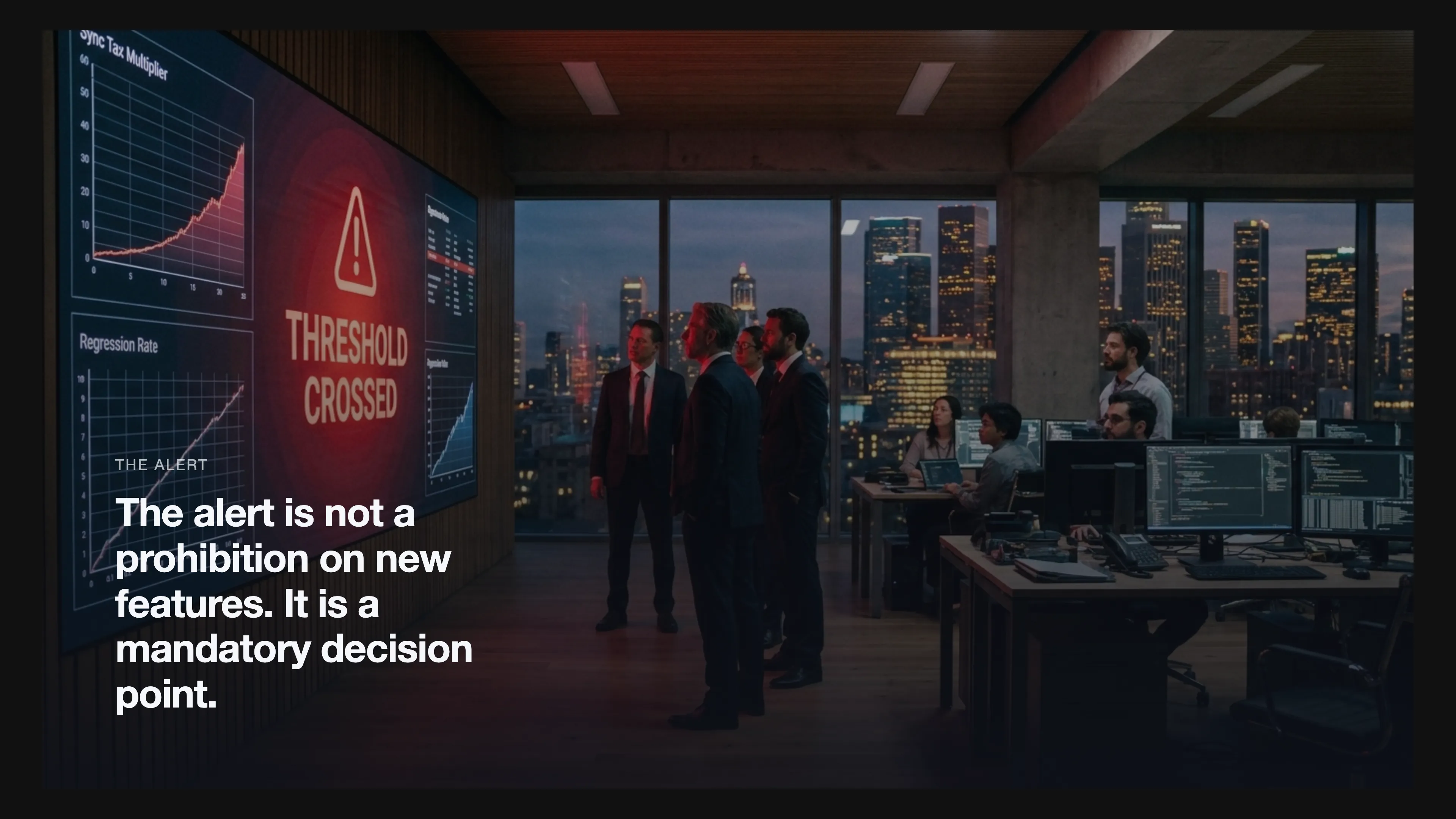
The Efficiency Metric is a public part of how the company operates. When the Sync Tax Multiplier or the Regression Rate crosses a predefined threshold, the system fires an automatic alert. The alert is not a prohibition on new features. It is a mandatory decision point.

Two audiences see the alert at the same time:

• The CEO and leadership team get a top-line view of the multiplier, the regression rate, and which parts of the system are paying the most tax. They make the trade-off at the company level: do we keep paying a 400% tax on innovation, or do we prioritize removing complexity to restore margins?
• The responsible team gets the same data, scoped to the parts of the system they own. They act on the parts they can fix without waiting for permission, because the team closest to the code is the one that can move fastest on it.

The alert doesn’t freeze the company. It forces a decision, and puts in evidence the data to the people who can act on it at the right level.

References

1. Page-Jones, M. (1992). “Comparing Techniques by Means of Encapsulation and Connascence.” Communications of the ACM, 35(9). https://connascence.io/pages/about.html
2. Page-Jones, M. (1996). What Every Programmer Should Know About Object-Oriented Design. Dorset House. Wikipedia: Connascence
3. Ford, N., Parsons, R., Kua, P., & Sadalage, P. (2022). Building Evolutionary Architectures: Automated Software Governance (2nd ed.). O’Reilly Media. https://www.oreilly.com/library/view/building-evolutionary-architectures/9781492097549/