Every Change to Your System Risks Breaking Something That Was Working

Why Every Feature Costs More Than the Estimate

1. The Feature That Cost Twice Its Estimate

A CEO approved a feature, and the actual cost came in at nearly double the estimate. Nobody lied, and the estimate was honest. It just didn’t include the cost of everything the feature broke.

Every change to a complex software system carries a risk of regression, meaning a change that breaks something that was working before. At worst, a new payment flow can crash the checkout page, an updated search algorithm might corrupt the recommendation engine, and a refactored authentication module could lock out half the users. Regressions are a predictable tax on complexity, and the more interdependent the system, the higher the tax.

The cost of these regressions is measurable, and the way to measure it already exists. For centuries, insurance companies have priced risk using a simple model. This article applies that model to software, and it prices the risk from how the system is built today, with incident history used only to price how much a break costs.

2. How Insurance Companies Price Risk

In maintenance engineering and actuarial science, there’s a foundational model for pricing risk called Frequency-Severity. Insurance companies use it to price policies, and maintenance contractors use it to price service agreements.

Frequency is how often failures happen, and severity is how much each failure costs, so the formula captures the expected total cost of failure.

$\text{Expected Total Cost} = \text{Expected Frequency} \times \text{Expected Severity}$

When a factory expects 2 breakdowns per year and each one costs $50k, the expected annual cost comes to $100k. An insurer would then price a maintenance policy at $100k plus a profit margin.

Software needs the same two inputs, and they come from different places. The frequency, the likelihood that a change breaks something, comes from the architecture: how many other modules the change touches, and whether the change stays contained inside one module. The severity comes from incident records: what a break actually cost the company. Oddly, companies calculate neither. They absorb the cost and call it the price of moving fast. An insurer who priced risk this way would be out of business in a quarter. Software companies do it for decades and call it agile.

3. Pricing Likelihood From the Architecture

A change’s likelihood of causing an incident is a property of how the system is built when the change ships. It’s computable from three components with three different origins: one measured from the test suite, one read from the code, one cited from research. Counting past incidents can’t price it: a spotless record can hide a tangled mess one change away from an outage.

For each change about to ship, the review asks one question with two parts: does this change stay inside one module, or does it force other modules to move, and how many? The answer is the Connascence Degree $C_d$ that Article 5 defines. A change with $C_d = 0$ is contained: it touches nothing else, so there’s almost nothing to break. A change with $C_d \geq 1$ crosses module boundaries, and every connascent module it drags along is a place the break can land and then propagate, through interfaces that may be poorly defined. The likelihood $p$ prices the incident itself, propagation included. The forced companion work that $C_d$ represents is a different cost, already priced as $CDC$ in Article 5.

Component 1: the change’s own escape factor, $(1 - c_0)$. Run the coverage report, or better the mutation score, on the module the change touches. That number, $c_0$, is the share of defects in the module the suite would catch, so $(1 - c_0)$ is the chance a defect slips past the change’s own tests. A module at 80% coverage has an escape factor of 0.2, and mutation tools measure this more honestly than line coverage because they inject real defects and count how many survive.

Component 2: the base rate $\rho$ for the module’s class. An escaped defect still has to reach a customer before it becomes an incident, and $\rho$ is the probability that it does, for a module of this class. It’s the only input with no home in the repository, so it starts from population research (industry change-failure rates run in the 20-40% band; the NIST and regression references below). It lives as one visible teaching value per class: high for customer-facing money paths, low for internal tooling. The company replaces these values with its own accumulated data as it matures, and every reader can challenge a value instead of a formula.

Component 3: a break factor $b_i$ per dragged interface. Each connascent module the change drags along is another place a defect can land, so inspect its boundary. A contracted, name-coupled seam with tests at the boundary is a low-class interface, while shared state with value coupling and no seam tests is a high-class interface. Then read module $i$‘s coverage $c_i$ exactly as in Component 1, and compute its break factor:

$b_i = \rho_{\text{class}} \times (1 - c_i)$

Assembling the likelihood. The change causes an incident when it breaks on its own or through any dragged interface, so the survival probabilities multiply. A contained change ($C_d = 0$) prices at $p_0$ alone, and every dragged interface multiplies the survival chance, which is how coupling turns into likelihood:

$p = 1 - (1 - p_0) \times \prod_{i=1}^{C_d} (1 - b_i), \quad \text{where } p_0 = \rho \times (1 - c_0)$

A worked example. A change touches the payment module at 80% coverage and drags two connascent modules: Billing on a shared-state seam at 40% coverage, and Search on a contracted seam at 90% coverage.

Component	Calculation	Value
$p_0$ (payment, customer-facing class)	$0.4 \times (1 - 0.80)$	0.08
$b_{\text{Billing}}$ (shared-state seam, high class)	$0.4 \times (1 - 0.40)$	0.24
$b_{\text{Search}}$ (contracted seam, low class)	$0.1 \times (1 - 0.90)$	0.01
$p$ assembled	$1 - 0.92 \times 0.76 \times 0.99$	$\approx 0.31$

For contrast, a contained change in a well-tested isolated module ($c_0 = 0.95$, $C_d = 0$) prices at $p_0 = 0.4 \times 0.05 = 0.02$, the near-zero intuition made arithmetic.

Two rules keep the calculation honest. One customer-facing outage is one incident, and the engineering hours inside it cover every break that caused it. And when a shipped change does cause an incident, the post-mortem checks the base rates: was the class right, and was the value honest? Incidents refine the values over time. They never set the structure, so a module with no history prices from its seams and its coverage, not from an empty record.

4. Pricing Severity From Incident Records

Severity is the one input where history earns its place, because a past incident is the only honest record of what a break costs end to end. For each incident $i$ in the records, compute the realized cost from that incident’s own logs:

$c_i = (t_{detect} + t_{fix} + t_{validate}) \times r + \text{revenue lost} + \text{churn} + \text{SLA penalties}$

$t_{detect}$ is the hours from the break to identification, $t_{fix}$ the hours to write and deploy the fix, $t_{validate}$ the hours to verify and monitor, and $r$ the blended hourly rate of the engineers involved, overhead included. One component was deliberately removed from earlier versions of this model: the opportunity cost of engineers fighting fires instead of building features. Those hours are already priced in $C_{eng}$, so adding their lost output on top counts the same hours twice. If the lost output matters more than the wages, replace the wages with the value of the lost output. Adding both is the error.

The expected severity $\hat{C_f}$ is the mean of the $c_i$ values, kept per incident class, because a cross-module incident (more hours, more business loss) and a contained incident are different animals:

$\hat{C_f} = \text{mean of } c_i \text{ per class}$

A company with no incident records yet can’t take that mean, so it estimates instead: engineering hours from the fix effort a typical break would need, plus the business loss the CEO expects from a day of degraded service. The estimate gets replaced by the first real $c_i$ values as they land, which keeps severity the only history-based input in the model.

5. Building the Multiplier

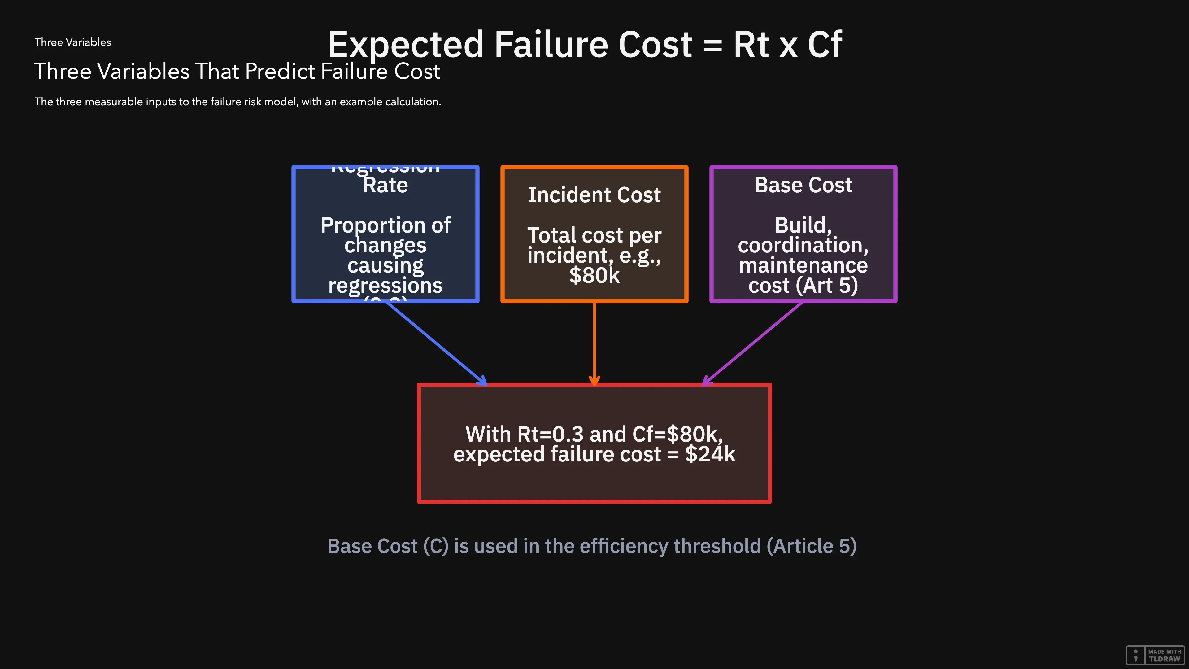
The last input is the exposure: $n$, the number of changes about to ship, whether that’s one change, one feature, or one quarter of shipping. With likelihood from the architecture, severity from the records, and the exposure stated, the failure risk cost of the change program is:

$\text{Failure Risk Cost} = n \times p \times \hat{C_f}$

This is the cost of the likelihood of an incident that hasn’t happened yet. The architecture says how likely, the records say how much, and $n$ says how many chances the system gets. History never appears in the likelihood, so a pristine tangled module still prices high, and a battered isolated module still prices low.

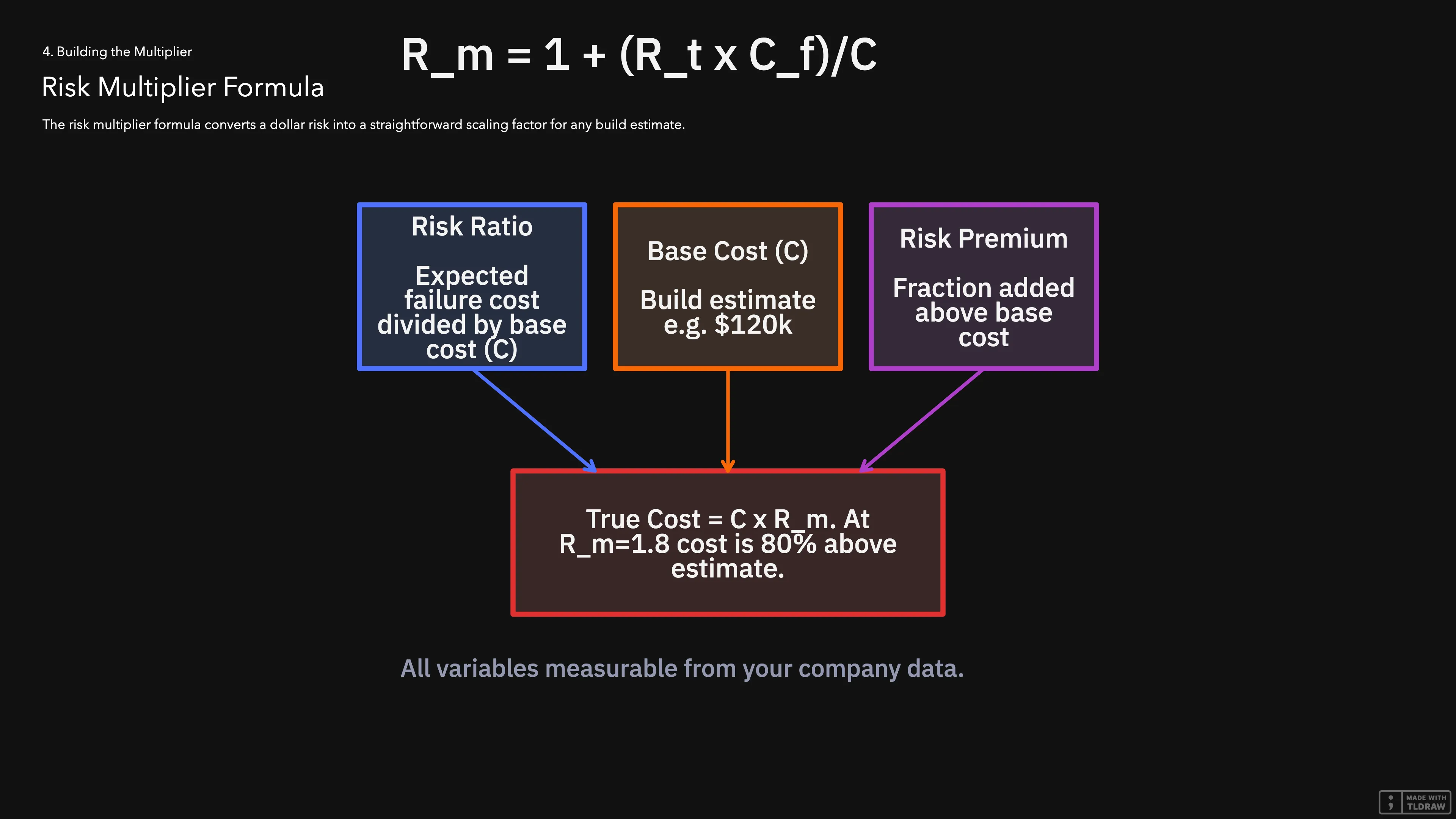
CEOs think in multipliers, so the risk gets expressed as a proportion of the base, with $n$ and $\mathbb{C}$ sharing the same scope. The cost of complexity $\mathbb{C}$, from Article 5, is what that same exposure costs to build and maintain if nothing ever broke: development, coordination, maintenance, and infrastructure.

$R_m = 1 + \frac{n \times p \times \hat{C_f}}{\mathbb{C}}$

$T\mathbb{C} = \mathbb{C} \times R_m = \mathbb{C} + (n \times p \times \hat{C_f})$

The second form is the honest identity: what you pay to build and maintain, plus what you expect to pay when it breaks. The multiplier is that same identity presented as a ratio, which is also why the additive form stays primary, since it keeps working when $\mathbb{C}$ is zero (section 7).

A worked example, with the exposure stated explicitly: a change profile that drags coupled modules prices at $p = 0.3$, and the cross-module incident class averages $\hat{C_f} = \text{\char"24}80\text{k}$, giving $24k of expected failure cost per change. With those numbers, a feature that ships as $n$ changes carries $n \times \text{\char"24}24\text{k}$ of expected failure cost, so $R_m = 1 + \frac{n \times \text{\char"24}24\text{k}}{\mathbb{C}}$, with $\mathbb{C}$ covering that same feature. The comfortable reading of this example, a $120k feature with a 1.2x multiplier, only holds when the feature is one change ($n = 1$) and the $120k is that change’s full cost of complexity, not the raw build estimate. Before trusting any multiplier, state $n$, because a feature is rarely one change.

6. Who Owns Which Number

A formula on a whiteboard is worthless if the people who need it can’t compute it. Specifically, the inputs live in different parts of the company.

The CTO owns the architecture and the engineering metrics.

The CTO computes $p$ per change from the three components: coverage and mutation scores from the test suite, boundary classes from the seam review, and the base-rate values the company maintains. From post-mortems and time logs, the CTO calculates $C_{eng}$ for each incident. These are hard numbers derived from the system and operational data.

The business impact belongs to the CEO.

For each incident, $C_{biz}$ comes from finance, CRM, and support systems. $\mathbb{C}$ comes from the CEO as well, because the cost of complexity grows out of the project budget and the operational spend. These are business numbers that engineering can’t measure.

How the handoff works.

The CTO brings the computed $p$ and $C_{eng}$, the CEO brings $C_{biz}$ and $\mathbb{C}$, and together they compute:

$\hat{C_f} = \text{mean of }(C_{eng} + C_{biz}) \text{ per incident}$

$R_m = 1 + \frac{n \times p \times \hat{C_f}}{\mathbb{C}}$

$T\mathbb{C} = \mathbb{C} \times R_m$

If the multiplier is 1.8, the CEO knows the true cost of the feature is 80% higher than its pre-risk cost. It’s an economic analysis that forces a better decision.

7. Where the Formula Breaks

Formulas break when reality doesn’t match their assumptions, so here are the edge cases and how the structural model handles each.

A zero base ($\mathbb{C} = 0$). When a change costs nothing to build, like a config toggle or a permission flip, it still carries risk, and the additive identity carries it directly: $T\mathbb{C} = n \times p \times \hat{C_f}$. The multiplier is the wrong presentation for a zero base, and the identity never needed the division in the first place.

A new system with no history. The likelihood needs no incidents, because the architecture review prices it. Severity is estimated from expected fix hours plus the CEO’s business-loss estimate, and the first real incidents replace the estimate.

A spotless record. Zero incidents in the logs don’t mean zero risk. A tangled module with a clean quarter still prices at its structural likelihood, which is the point: the past can’t zero out what the architecture can still break. The flip side matters too, since a coupled module that never broke prices high while it stays coupled, so the only way to lower its price is to actually decouple it.

Correlated breaks. Three breaks that share one customer-facing outage are one incident, one $c_i$, and one business loss, which is why the model never multiplies one outage’s revenue loss by three. The incident unit handles correlated risk by construction.

Scope confusion and stale inputs. $n$ and $\mathbb{C}$ must describe the same exposure: per feature for decision-making, per quarter for trend analysis, always labeled, because a per-change failure cost divided by a quarterly base produces a number that means nothing. The inputs re-read cheaply: coverage and boundary classes come from the repo as it stands when the change ships. Base rates age slowly, so incidents refine them after the fact, and a class assignment that keeps missing real coupling gets fixed, not averaged away.

8. The Cost Nobody Owns

The industry doesn’t calculate incident costs properly. Engineering tracks downtime and mean time to recovery. Finance tracks the revenue impact in its own ledger, and support tracks tickets in its own queue. The cost of poor-quality software in the US alone has been estimated in the trillions, yet each department owns a fragment of the cost, and the total has no defender.

CEOs make bad decisions because the total cost is invisible. The risk multiplier brings it into the open, and it prices risk the way an insurer would: from what the system is, not from what the logs happen to show. Once visible, something else happens: the formula creates incentives to reduce the numbers that feed it.

When most changes price at a high $p$, the multiplier is high, and every feature decision carries a visible risk premium. That premium creates pressure to lower $p$, and lowering $p$ means making architectural choices that isolate components from each other, so a change in one place doesn’t cascade into three others. The premium pays for decoupling, and decoupling is the only durable way to stop paying it.

The alternative is approving features based on vibes and hoping the regressions sort themselves out. That strategy has a perfect record of not working.

Before a CEO approves a feature, the risk premium belongs on the table next to the estimate. If the premium is 80%, he might choose a safer architecture or kill the feature. If it’s 10%, he proceeds with confidence. Either way, economics drives the decision, not gut feeling.

References

• Software Regression. Wikipedia
• Frequency-Severity Method. Investopedia
• Why Bug Fixes Introduce New Bugs: A Comprehensive Review of Regression Defects in Software Engineering. IJS RET, 2026
• The Cost of Poor Quality Software in the US: A 2022 Report. CISQ
• Site Reliability Engineering. Google (Chapter 1 - Introduction)
• The Economic Impacts of Inadequate Infrastructure for Software Testing. NIST, 2002