Coupling Isn't a Binary Switch, and Every Level Has a Price

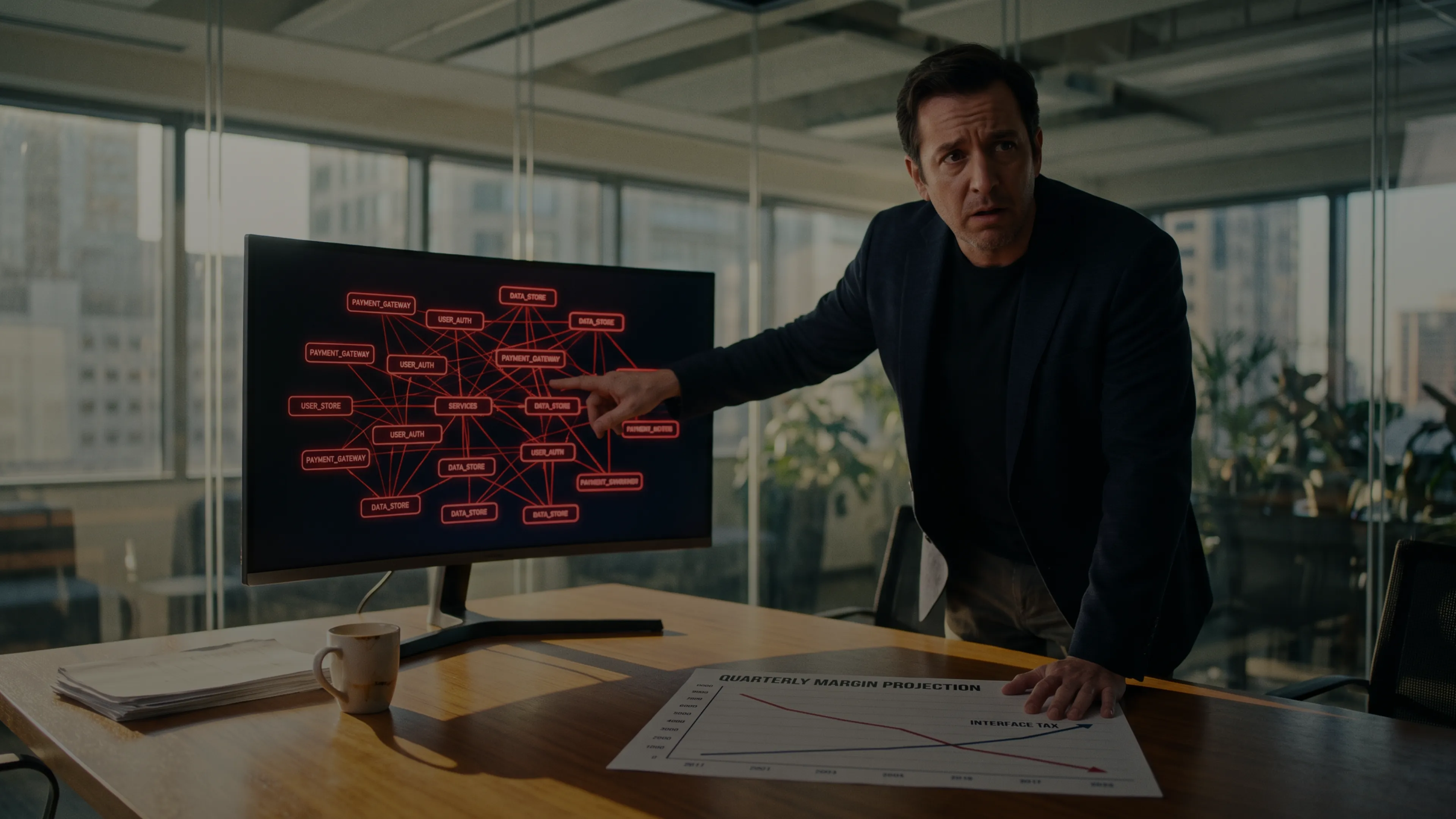
Every Interface Decision Has a Hidden Bill

1. The Gap in Interface Thinking

For software engineers, interface conversations center on technology: different communication protocols and message systems. Architects, meanwhile, frame the discussion around patterns: layered designs, event-driven flows, orchestration. Business leaders talk about outcomes: speed, cost, risk.

None of these conversations connect. An engineer picks a message broker because it reduces direct dependencies. Architects choose a layered architecture to isolate the core logic from external tools. A business leader, meanwhile, approves the budget without understanding that both choices will double the maintenance cost three years from now.

Tying everything together is connascence. Meilir Page-Jones invented connascence in 1996 as a measure of coupling, and Ford, Parsons, and Kua adopted it in Building Evolutionary Architectures. Two components are connascent when a change in one forces a change in the other. The more components that must change together, the higher the connascence, and the higher that cost climbs for every future feature.

Connascence is a metric, not a framework or taxonomy. It quantifies coupling and gives leaders visibility into the real cost of their interface decisions before they commit. This article connects each interface design choice to its connascence level, and connects that connascence level to the economic formulas from earlier articles: the Sync Tax Multiplier ($S_t$), the Failure Risk Multiplier ($R_m$), and the strangler extraction cost. You can see the price of your decisions before you make them.

2. Connascence: A Vocabulary for Coupling

When it comes to naming coupling, the software industry has a poverty of language. We say “tightly coupled” or “loosely coupled” as if coupling were a binary switch, but connascence gives us the precision the industry has been missing.

For every connascence relationship, Page-Jones defined three properties:

Property	Meaning
Strength	How hard the connascence is to discover and fix. Build-time coupling (tools catch it before production) is weaker. Runtime coupling (users catch it after production) is stronger. Even the weakest runtime coupling is stronger than the strongest build-time coupling, because build-time problems never reach a customer.
Locality	How far apart the connascent elements are in the code. Closer is better.
Degree	How many elements share the connascence relationship. More is worse.

The connascence types fall into two categories, from weaker to stronger:

Build-time coupling (cheaper, caught by tools before production): At build time, these are agreements about the names of functions and data fields, the type of data each component expects, the order in which data is passed, algorithms, and the meaning of specific values. If two components disagree, the compiler or automated tests catch it before anyone ships. The cost is low because the problem never reaches a customer.

Runtime coupling (expensive, caught by users after production): At runtime, these become agreements about execution order, timing, shared values, and shared references to other components. If two components disagree here, nobody finds out until a customer hits the bug in production. The cost is high because the problem reaches the market.

For precise classification, engineers can refer to the full nine-type taxonomy from Page-Jones and Building Evolutionary Architectures.

The core rule from Ford, Parsons, and Kua in Building Evolutionary Architectures: “Strive for weak connascence between modules, allow strong only inside the module”.

Within a domain, controlled by a single team, high connascence is acceptable when it serves customer demand. Across domains, where different teams own different bounded contexts, connascence must be minimized. Every dimension of interface design either increases or decreases one of these connascence types.

The goal is not zero coupling. Some coupling serves customer demand and is worth the cost. A payment system that calls fraud detection synchronously is coupled, but that coupling exists because the business needs fraud checks before payment. The goal is to see which coupling is appropriate and which is accidental, then decide whether the cost is worth paying.

3. Dimension 1: Visibility

In Design Rules, Baldwin and Clark showed that modularity depends on separating visible design rules from hidden parameters. Visible design rules are the interfaces everyone must obey. Hidden parameters are the internals each module controls independently.

Good: IBM System/360. By publishing the interface specification for every peripheral manufacturer, IBM made the design rule visible. That visible design rule became the contract anyone could depend on. Inside each peripheral, engineers changed circuits freely without telling anyone. As long as they still spoke the published interface protocol, innovation stayed hidden behind the boundary. The interface served as the stable anchor. Internals stayed unknown to consumers. Connascence between the system and its peripherals was Name and Type only, the weakest forms.

Bad: A team publishes an internal library with a “stable” public API, but the library itself exposes internal classes as public methods because it’s easier. Another team starts depending on those internal classes. The library team changes an internal method. Three other teams break. The “visible” boundary was never actually visible, everything leaked. The connascence exploded from Name and Type to Algorithm and Position without anyone noticing.

Economic question: Did the second team save time by reusing an internal class? In the short term, yes. In the long term, every library change will now trigger coordination meetings, regression testing across three teams, and delayed releases. The Sync Tax Multiplier ($S_t$) just increased because the Connascence Degree ($C_d$) went from 0 to 3.

4. Dimension 2: Domain Scope

For the definitive guide here, look to Domain-Driven Design’s bounded context. At its core, a bounded context is a boundary where the same business concept has one clear meaning and one team owns it. Different contexts give the same word different meanings. “Customer” in billing is not the same thing as “customer” in fulfillment.

Good: In the Transactions domain, the Payments module calls Fraud Detection synchronously. Since both belong to this same domain, the same team owns the coupling and pays the cost. When Fraud Detection changes its internal scoring model, Payments adapts in the same sprint. High connascence appears here (Execution and Timing, the strongest runtime types), but the cost stays low because the domain boundary contains it. Because the business requires this coupling, it serves a real purpose: fraud detection must happen before payment, so the connection serves a real purpose.

Bad: Consider three contexts consuming a single CustomerUpdated event: CRM, Billing, and Support. CRM interprets “customer” as a prospectable party. For Billing, it means a financially accountable account. Support reads it as a person with an open case, creating three incompatible meanings from one event. Adding a field for one receiver breaks another. Without a single team owning all three interpretations, nobody can fix it. A domain must be owned by a single team. If multiple teams share a domain boundary, Conway’s Law will make them pay.

Economic question: Did the sender save time by broadcasting one event instead of building three purpose-built interfaces? Yes, in the first sprint. Every future change to that event now requires coordination across three teams, three contexts, and three sets of business rules. In the Sync Tax formula, the Coordination Overhead ($C_{coord}$) just multiplied by three.

5. Dimension 3: Direction

In the Ports and Adapters pattern, Alistair Cockburn distinguishes two directions of communication: primary ports, what the outside world calls to use your system, and secondary ports, what your system needs from the outside world. Under this pattern, a port is a contract your system defines. An adapter is the specific tool that fulfills that contract. Your system defines what it needs, and then a specific vendor takes over with an implementation. Swap the adapter, and the port doesn’t change. The critical rule: “Never explicitly name any external object or technology. Always take a parameter for any external object or technology you wish to access”.

Good: Picture a payment gateway exposing a “process payment” interface as a primary port. Clients in the outside world call it. The core domain defines a “send order confirmation” interface as a secondary port, a contract the domain owns and controls. Email tools implement it. Swap email for SMS, and the core doesn’t change while control over the secondary port’s contract stays with the domain. Only Name and Type connascence remains, owned by the domain.

Bad: Instead of defining its own port, the core domain calls the email vendor’s function directly. When the email vendor changes its API, the core domain breaks. The domain didn’t define what it needed. It coupled itself to what a vendor offered. Identity and Algorithm connascence now bind both sides together (the domain and every consumer share the same email vendor dependency and must match the vendor’s specific API pattern).

Economic question: Did the team save time by skipping the port abstraction? In the month they shipped, yes. When the email vendor changed their API and the team spent two weeks rewriting every integration point instead of one adapter, the Sync Tax collected its payment.

6. Dimension 4: Synchronicity

With a synchronous call, the caller is chained to the called. Availability, response timing, and contract agreement must hold on both sides. A synchronous interface creates Connascence of Execution and Timing. These are the two strongest runtime connascence types. When you call synchronously across a domain boundary, you couple your service’s availability to another team’s service. Good: Consider ecommerce checkout publishing OrderPlaced asynchronously. Payment, inventory, fraud, and email consume it independently, with checkout returning success almost instantly. If email is down, orders still process while later draining from queues. Only where the caller genuinely needs an immediate answer, like validating a credit card before confirming the order, is a synchronous call used. Even then, the dependency is measured and explicitly accepted.

Bad: In a single request chain, checkout calls inventory, payment, fraud, and email synchronously. 95% of requests take 630 milliseconds or more, before any actual business logic runs. If any one service is down, every order fails. The availability of the entire business is the product of four services’ individual availability: $0.999^4 = 99.6\%$. One slow downstream drags every customer into the same wait. At the fourth service, a single timeout wastes all the work done by the first three.

Economic question: Easier to build, the sync chain offered short-term gains. Yet the Coordination Overhead ($C_{coord}$) in the Sync Tax formula now includes every latency spike, every timeout, every retry, and every on-call incident caused by a downstream service that was not the caller’s responsibility.

7. Dimension 5: Contract Formality

How strict an interface contract is determines how many connascence types stay active and whether tools catch them at build time or users catch them at runtime. A strict contract limits connascence to Name and Type. A tolerant contract (or no contract at all) invites Algorithm, Position, Value, and Identity.

Good: Two teams agree on a strict, machine-verified contract. Designed so adding new fields doesn’t break existing consumers, the contract protects downstream systems. Fields they don’t recognize are simply ignored by older systems. Machine verification enforces the contract. Automated quality checks reject any change that breaks backward compatibility. With each schema version, both teams coordinate only on the fields they actually share, leaving room to evolve independently. Name and Type connascence, verified at build time, is the result.

Bad: Consider multiple services sharing the same database. Orders writes to the orders table while Shipping reads from it directly, so when Orders changes a data field type, Shipping breaks at runtime with no warning. Without any contract, versioning, or governance, the teams operated blindly. That “tolerance” was just blindness to the coupling. Connascence of Value and Identity are now active, and they’re the strongest types.

Economic question: Free during development, the shared database created hidden costs. Now the Regression Rate ($R_t$) includes every runtime error from a database structure change that propagated incompletely. The Failure Risk Multiplier ($R_m$) captures the cost of those regressions. If $R_t = 0.2$ and each regression costs $50k to fix, every feature carries a $10k expected failure cost on top of its build cost.

8. Dimension 6: Communication Pattern

How coordination is owned and how many consumers a change affects both depend on the communication pattern.

Good: With OrderPlaced, inventory reservation, analytics indexing, and search indexing all trigger simultaneously via events. Who consumes the event is unknown to the sender. Each receiving system acts independently. Without touching the sender, a new receiver subscribes. The event schema keeps connascence at Name and Type, so the Connascence Degree ($C_d$) for the sender is zero.

Bad: When a checkout service needs to know if inventory is available before confirming an order, the team has options. Instead of calling a “check stock” function synchronously and getting an answer in 50 milliseconds, the team publishes an InventoryCheckRequest event, subscribes to InventoryCheckResponse, and matches each request with its response by ID. The caller needed an immediate answer. Now it has a messaging system, logic to match each request with its response, timeout handling, and data that aligns eventually but not immediately, all solving a problem that a direct call would have solved with one line.

Economic question: Did the team avoid coupling? No. They traded synchronous Execution connascence for asynchronous Execution connascence plus a new Identity connascence on the matching ID. From the direct call to the messaging system, the complexity moved but it did not disappear. Compounding with every new engineer who needs to understand it, the maintenance cost of the matching logic grows.

9. Dimension 7: Coordination

Who knows the workflow and who pays for debugging are determined by orchestration and choreography.

Good: In a payment transaction, an Order Workflow Orchestrator manages the flow: sends “create order”, then on success sends “process payment”, then on success sends “reserve inventory”, then on success triggers shipping. If payment fails, it sends reverse actions that undo previous steps.

The entire workflow lives in one service. Debugging a failed order means looking at one place, and concentrated there, the orchestrator holds the connascence of Execution.

Bad: Through events only, multiple services choreograph a payment workflow. Order publishes OrderCreated. Payment consumes it, processes, publishes PaymentProcessed. Inventory consumes that, reserves stock, publishes InventoryReserved. If a customer’s order fails at step three, no single service knows why. Across four separate systems, the workflow is spread. Debugging requires tracing events through a messaging system with no single source of truth.

Economic question: By eliminating the orchestrator’s Execution connascence, choreography distributed the operational cost across every team involved in the workflow. When an order fails in production, which team investigates? How many engineers spend how many hours tracing a failure that the orchestrator would have caught and reported in seconds? From build time to runtime, the Coordination Overhead ($C_{coord}$) shifted.

10. From Connascence to Cost

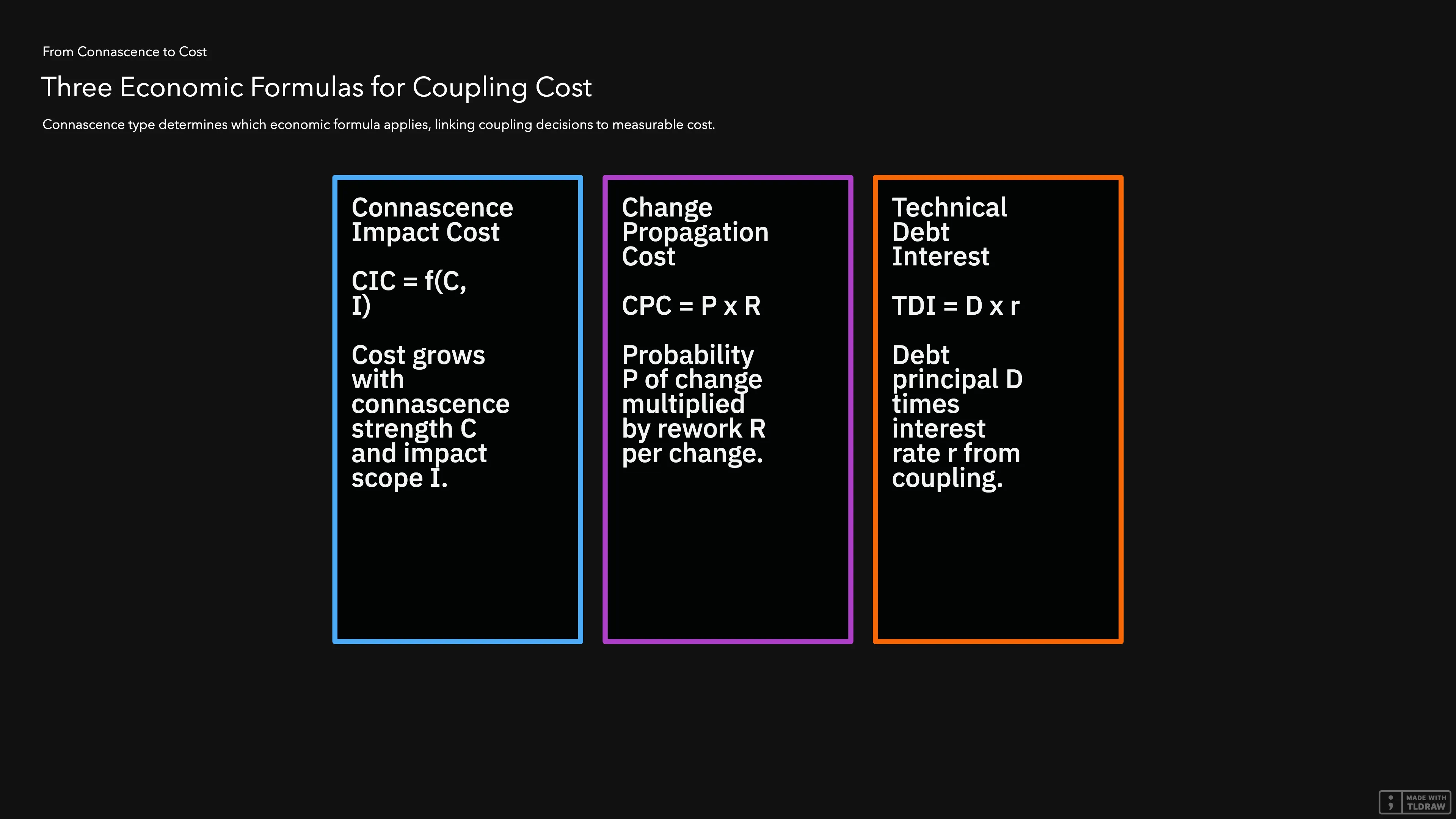
When you make a dimension choice, you increase or decrease a specific connascence type. That connascence feeds into three economic formulas from earlier articles. Here is each formula with what it measures and which connascence types drive it.

Formula 1: Sync Tax Multiplier ($S_t$)

What this formula measures is each feature’s extra effort cost from coupling. It comes from Article 9.

The terms:

• $E_v$ (Vacuum Effort): Hours a task takes in a perfectly isolated module, with no dependencies. This is your baseline cost.
• $k$ (Interdependence Factor): How much each dependent module adds to the effort, as a fraction of $E_v$. Default 0.5, meaning each dependent module adds 50% of the original effort.
• $C_d$ (Connascence Degree): How many other modules must change when one module changes. This is the Degree property from Page-Jones’s framework.
• $C_{coord}$ (Coordination Overhead): Hours spent in meetings, reviews, and cross-team communication to align changes.

The formula:

$S_t = 1 + k \cdot C_d + \frac{C_{coord}}{E_v}$

Connascence mapping: $C_d$ captures Identity and Algorithm (how many components share a dependency). $C_{coord}$ captures Execution and Timing (synchronous calls force order and time constraints). Together they multiply the cost of every feature.

Formula 2: Failure Risk Multiplier ($R_m$)

How much your system’s fragility costs per change is what this formula measures. It comes from Article 5.

The terms:

• $R_t$ (Regression Rate): How often a change in one component breaks an unrelated component. Measured from historical incident data.
• $C_f$ (Incident Cost): Total regression cost: engineering fix time plus business impact (lost revenue, customer churn, SLA penalties).
• $\mathbb{C}$ (Complexity Cost): The total cost of complexity before risk, calculated as $(CDC + STC) + ECC$ from Article 5.

The formula:

$R_m = 1 + \frac{R_t \times C_f}{\mathbb{C}}$

Connascence mapping: $R_t$ is driven by Connascence of Value. When two components must maintain synchronized values and they diverge, the system breaks. Higher $R_t$ means higher expected failure cost on every change.

Formula 3: Strangler Extraction Cost ($C_{total}$)

The cost of transitioning to modularity, when changes aren’t frozen during extraction, is what this formula measures. It comes from Article 19.

The terms:

• $ETC$ (Extraction Team Cost): Monthly cost of the engineers building the new module.
• $T$ (Duration): Months the old and new systems run in parallel.
• $C_{sync}$ (Sync Cost): The monthly cost of maintaining the data bridge between old and new systems if it were a simple pipe with no transformations.
• $S_t$ (Sync Tax Multiplier): From Formula 1, applied to the sync layer.
• $\mathbb{M}$ (Magnitude Multiplier): How much harder the actual sync layer is compared to a simple pipe. Measured as actual sync effort divided by ideal sync effort. When $\mathbb{M} = 1$, the sync just copies data. When $\mathbb{M} = 4$, the sync demands four times the effort of a simple pipe.

The formula:

$C_{total} = (ETC \times T) + (C_{sync} \times T \times S_t \times \mathbb{M})$

Connascence mapping: the sync layer is pure connascence. What $\mathbb{M}$ measures is the cost of maintaining Connascence of Value across two divergent schemas. Every product change during extraction increases the divergence, which increases $\mathbb{M}$, which multiplies the total cost.

Connascence Degree Cost: Translating Coupling to Money

Through code-analysis tools that tally unrelated files or modules touched by a change, the Connascence Degree ($C_d$) counts how many components share a dependency. A high $C_d$ mathematically proves interdependence. It is the cold, hard number that replaces gut feelings about coupling with something a business leader can act on.

Converting connascence into money is the role of the Connascence Cost ($CDC$) formula. The terms:

• $C_d$ (Connascence Degree): Number of components sharing a dependency.
• $k$ (Interdependence Factor): How much each dependent module adds to the effort, as a fraction of $E_v$.
• $E_v$ (Vacuum Effort): Hours the task takes in isolation.
• $R$ (Blended Hourly Rate): The fully loaded cost of an engineering hour.

The formula:

$CDC = C_d \cdot k \cdot E_v \cdot R$

If $C_d = 3$, $k = 0.5$, $E_v = 20$ hours, and R = \120$:

$CDC = 3 \cdot 0.5 \cdot 20 \cdot 120 = \$3,600$

On top of the feature’s own build cost, that’s $3,600 in extra cost, purely because three modules share a dependency. That cost is the Sync Tax. Every interface dimension choice either increases or decreases that number.

Summary: How Each Dimension Feeds the Formulas

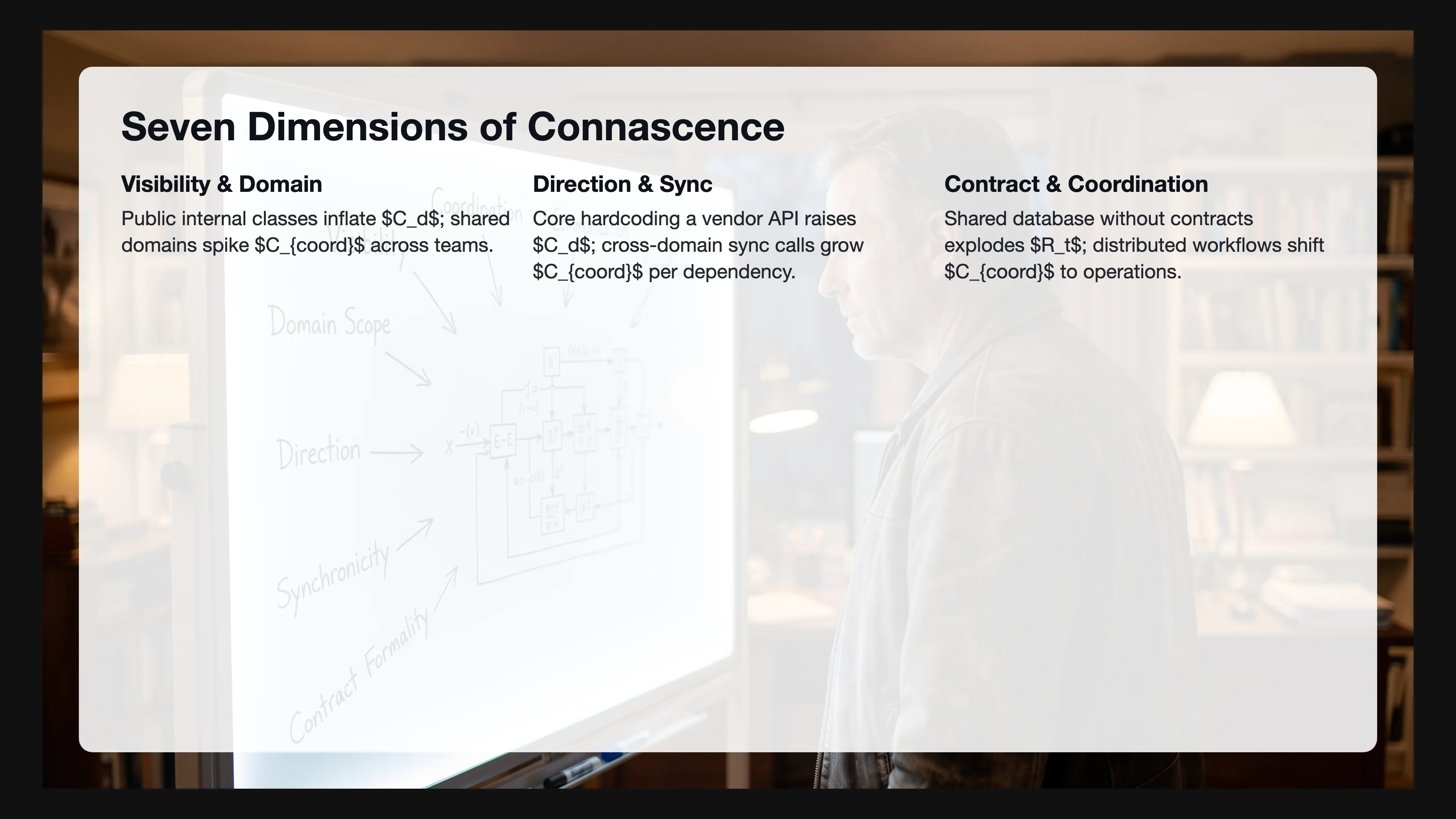
How each dimension choice feeds into the formulas above is summarized in this table.

Dimension	Choice That Increases Connascence	Connascence Type	Formula Impact
Visibility	Internal classes leaked as public	Algorithm + Position (build-time)	$C_d$ inflated: every consumer becomes a dependent
Domain Scope	Shared domain across teams	Even Name/Type is risky	$C_{coord}$ spikes: different teams, different priorities
Direction	Core hardcodes vendor API	Identity + Algorithm	$C_d$ includes every integration point with the vendor
Synchronicity	Cross-domain sync call	Execution + Timing (runtime, most expensive)	$C_{coord}$ grows per dependency in the chain
Contract Formality	Shared database, no contract	Identity + Value (runtime, most expensive)	$R_t$ explodes: database structure changes in one place but not the other
Communication	Sync work disguised as async	Identity (matching ID) + Execution	$C_{coord}$ shifts but doesn’t disappear
Coordination	Distributed workflow, no owner	Execution spread across teams	$C_{coord}$ shifts from build to operations

11. Conclusion

Every interface design choice is an economic decision implemented by technology. Synchronous or asynchronous, orchestrated or choreographed, strict or tolerant, each choice sets a connascence level that will compound for the life of the system.

The formulas are where connascence finds its financial expression. $S_t$ tells you how much your coupling choices cost per feature. $R_m$ tells you how much your fragility costs per change. How much the transition to modularity will cost if you don’t freeze changes during extraction, the strangler extraction formula tells you.

None of this requires new formulas because the bridge already exists: connascence is the measure, and the formulas translate that measure into cost. When you choose an interface type, you’re choosing a connascence level, and choosing a connascence level means choosing how much tax you’ll pay on every feature from now until the system is modularized.

For every leader, the question is practical: if we make this choice now, will the product still be feasible in the foreseeable future? The answer is unique to every situation. This article gives leaders the visibility to see the real cost of each option rather than prescribing one interface type over another. When that cost becomes visible, reducing complexity becomes economically convenient. Leaders allocate resources to fix coupling when they can see that the alternative is bankruptcy.

Business leaders don’t need all nine connascence types. What they need is one number: $C_d$, the Connascence Degree. When that number goes up, everything gets exponentially more expensive. When it goes down, margins improve. The seven dimensions in this article are the levers that control that number.

References

1. Page-Jones, M. What Every Programmer Should Know About Object-Oriented Design. Dorset House, 1995. See connascence.io for the full taxonomy and history.
2. Ford, N., Parsons, R., Kua, P., Sadalage, P. Building Evolutionary Architectures, 2nd Edition. O’Reilly, 2022. O’Reilly catalog page.
3. Baldwin, C.Y., Clark, K.B. Design Rules, Volume 1: The Power of Modularity. MIT Press, 2000. MIT Press.
4. Cockburn, A. “Hexagonal Architecture (Ports and Adapters)”, 2005. alistair.cockburn.us.

Measure it

Price the coupling level on this interface

Skipping the port abstraction saved time in the month the team shipped. The vendor API change then took two weeks at every integration point, and the calculator prices that coupling on the next change.

• Price this interface's coupling →
• See this coupling cost in Defusor →