The Cost of the Shortcut Compounds Non-Linearly, and Nobody Sees It

Showing Business Leaders the Future Cost of Today’s Shortcuts

A feature request arrived in a planning meeting, and engineering estimated four weeks to do it right, but leadership pushed for two. Engineering cut corners, skipping the debt cleanup, deferring the interface work, and reducing the testing, and the feature shipped on time, with everyone celebrating as if the cost never existed.

This article describes a simulation that makes those invisible installments visible by using the formulas introduced in previous articles to project cost trajectories. So business leaders can see the divergence between the disciplined path and the fast path before they choose.

1. How the Fast Path Happens

The dynamic is counterintuitive: engineering didn’t walk into a planning meeting and offer two options with different timelines. Engineering proposed the right way, leadership pushed hard to move faster, and engineering, under pressure, started offering cheaper versions. The fast path came from that pressure, and engineering conceded because leadership demanded a faster timeline than the disciplined approach allowed.

The simulation models this honestly. Path A is what engineering would have done if given the budget, and Path B is what happened after the negotiation. Path A did the cleanup work that kept components evolving independently, then built the new feature with proper interfaces, and complexity stayed at the same level. Path B implemented as fast as possible, no matter what happened to the architecture, which made it cheaper that day but catastrophically more expensive over time.

2. What the Fast Path Hides

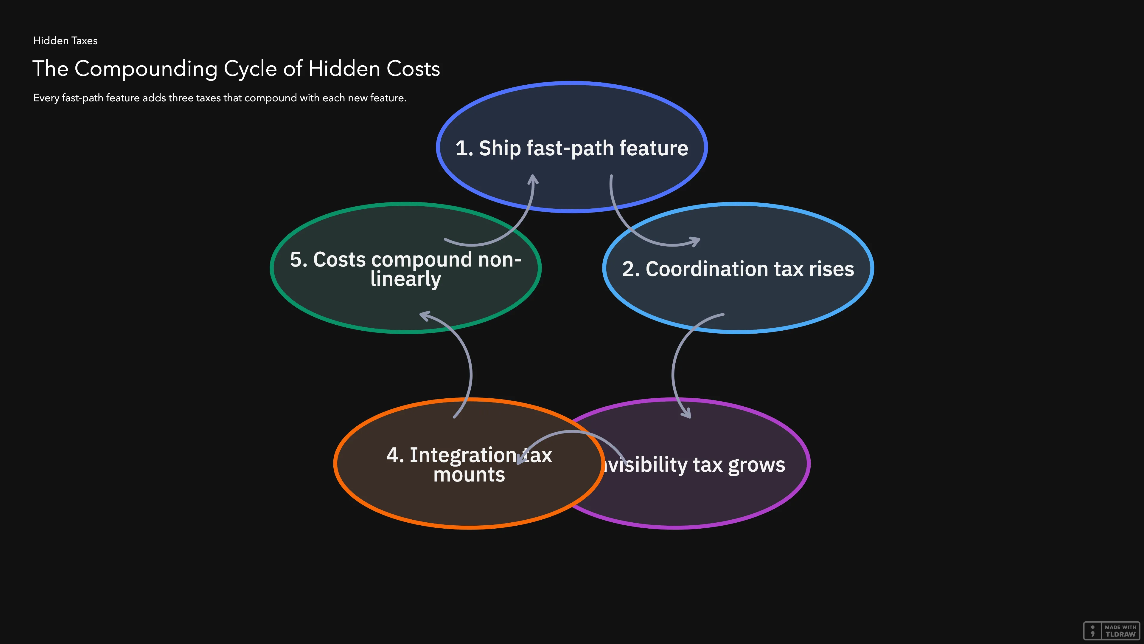
Every fast-path feature creates three hidden taxes on the engineering organization, and the costs compound with every additional feature shipped the same way.

The coordination tax comes from skipping the interface work, sharing databases, and baking assumptions into the code, all of which create new links between parts of the system. The next change has to coordinate with another team, which means more meetings and more time spent waiting for alignment.

A minor data format change in one part of the system can cascade into failures in other parts when teams haven’t defined clear rules for how the parts should connect. The same shortcut that saves two weeks during implementation creates a permanent risk that compounds with every future change.

The invisibility tax is the most dangerous because the implementation looks cheap on day one, while the bill arrives later, disguised as slower delivery, more incidents, and engineers who can’t explain why their velocity is dropping.

After a handful of fast-path features, the three taxes compound, and the system has accumulated enough hidden cost that every future feature costs more than it should. The compounding accelerates, so five fast-path features don’t just double the cost, they more than double it.

For business leaders, what matters is the dollar cost of the compounding, and the simulation projects that cost in three steps: measure the current state, model the future, compare the two paths. The full cost model lives in Article 9, but for the takeaway here, what matters is that the cost grows with every fast-path feature, and the growth is non-linear. The table in the next section shows the trajectory.

3. Cost Projections

The table below shows what the simulation produces, with the starting cost depending on the system’s current state. A system that has been disciplined for years starts near 1.0, meaning features cost what they should, but a system that has been shipping fast for years starts at 1.3 to 1.5. Meaning every feature already costs 30% to 50% more than it should.

Each row shows the cost multiplier after approving a given number of additional fast-path features, and a multiplier of 2.5x means a feature that should take 4 weeks actually takes 10 weeks.

Fast-path features approved	Cost multiplier (clean system)	Cost multiplier (typical system)
0	1.0x	1.3x - 1.5x
2	1.05x	1.4x - 1.7x
5	1.15x	1.8x - 2.2x
10	1.3x	2.5x - 3.5x
20	1.6x	3.8x - 5.5x

%%{init: {"themeVariables": {"xyChart": {"plotColorPalette": "#2CC48B, #E4A82C, #E42728"}}}}%%
xychart-beta
    title "Cost Multiplier by Fast-Path Features Approved"
    x-axis [0, 2, 5, 10, 20]
    y-axis "Cost Multiplier (x)" 0 --> 6
    line "Clean system (1.0x start)" [1.0, 1.05, 1.15, 1.3, 1.6]
    line "Some debt (1.3x start)" [1.3, 1.4, 1.8, 2.5, 3.8]
    line "Years of debt (1.5x start)" [1.5, 1.7, 2.2, 3.5, 5.5]

The green line represents a clean system, the orange line represents a system with some accumulated debt, and the red line represents a system with years of accumulated complexity. The clean system barely moves: twenty fast-path features push the cost multiplier from 1.0x to 1.6x. A system with some accumulated debt doubles within ten features and more than doubles within twenty. A system with years of debt starts at 1.5x and ends at 5.5x, which means every future feature costs more than five times what it should. Real systems typically fall between the orange and red lines, and the gap between a clean system and a debt-laden one widens with every additional fast-path feature approved.

4. What the Research Confirms

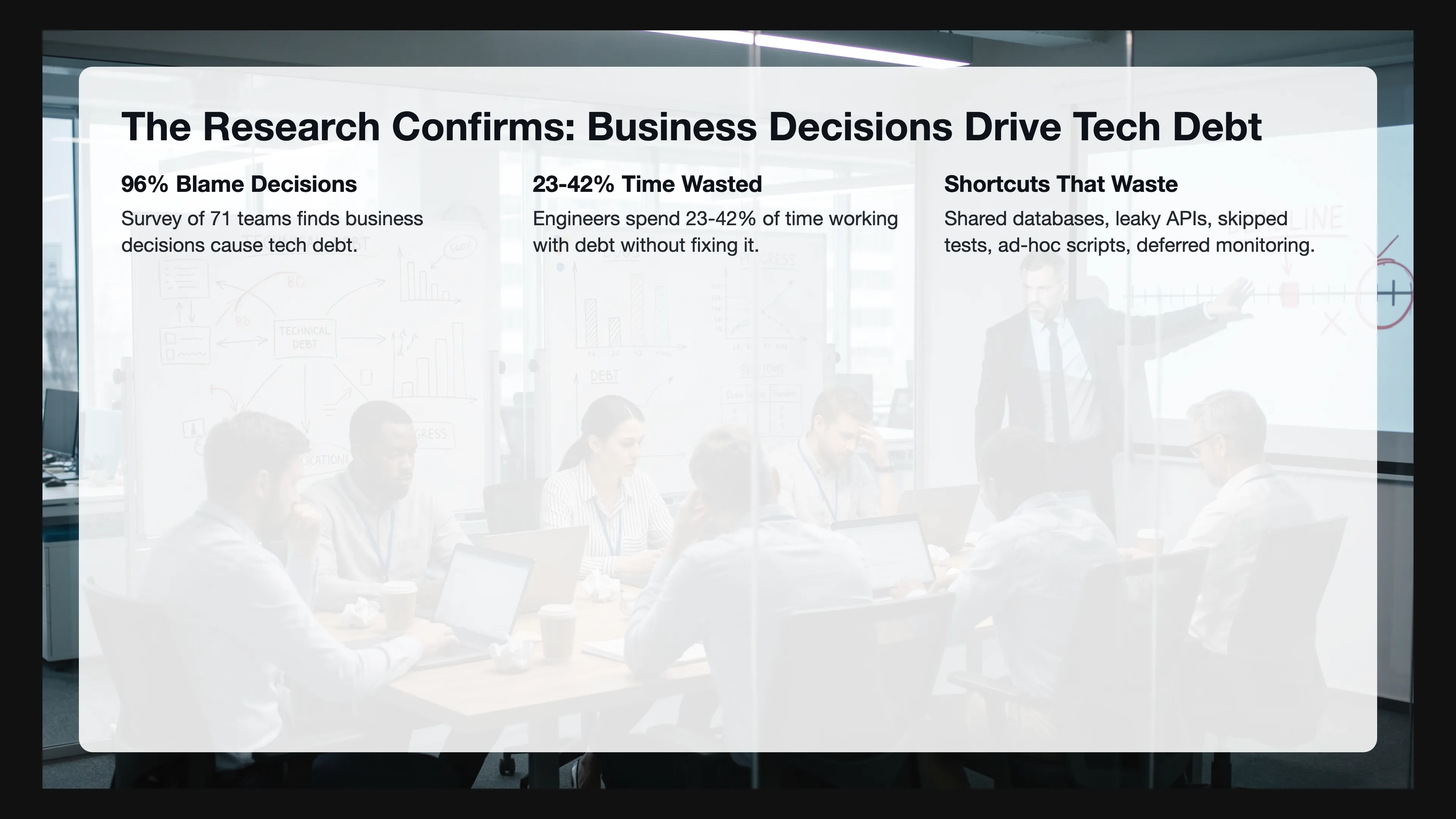
Survey research with 71 engineering teams (arXiv paper 2104.09330v5) found that 96% report business decisions directly contribute to technical debt creation. Tight deadlines are the #1 cause and features prioritized over quality are the #2 cause, and market pressure drives both.

Quantitative research measured the impact: engineers waste 23% to 42% of their time working with technical debt without fixing it. Changes in code with high debt density take 124% longer to complete than changes in healthy code, and the Maintainability Index drops 0.9% per month in repositories where debt density grows above 10% per year.

The shortcuts that create this waste are well-known: sharing databases instead of building APIs, building APIs but leaking internal logic and data, skipping tests on edge cases, baking assumptions into the code, and scattering business logic across ad-hoc scripts. Deferring monitoring and tracing is another shortcut that creates new connections, and each connection feeds the compounding tax, which is what the simulation projects as the dollar cost of these shortcuts compounding over time.

5. Diagnosis vs Prediction

The diagnostic metrics and the simulation serve different jobs, with one diagnosing the present and the other predicting the future, and confusing them defeats the purpose of both.

Diagnosis measures the current waste by looking at how many hours engineers spend in coordination meetings, how long it takes to fix problems when they occur, and how often changes break something else. Velocity as an absolute number is a vanity metric, and story points are even worse, but if you track velocity for the same engineer consistently across multiple quarters and the number drops, the engineer didn’t get slower. The system got harder to maintain, and once you translate those hours to currency using the average engineer cost, you get the current waste in monetary terms.

Prediction projects the future by taking the current state and asking what each quarter will cost us over the next two years if we approve the next six features the fast way. The leader who sees a prediction showing a widening gap between the disciplined path and the fast path can make a different decision than the leader who only sees the immediate price tag on a single feature.

6. Why This Matters Now

Article 22 established the Christensen timing framework: after product-market fit, the strategy must shift from emergent to deliberate, and the architecture must move from integrated to modular. Companies that miss this shift keep adding features the fast way to a system that can no longer absorb them.

The simulation makes that shift undeniable, because a leader looking at the typical-system projection sees that continuing emergent-mode feature delivery on top of an already complex system doesn’t just cost more, it breaks the economics of the business. Each quarter delivers fewer features at higher cost, margins compress, and competitors who modularized earlier capture the cost advantage.

Investors are getting more selective, and the era of subsidizing complexity with virtually unlimited capital is ending which means CEOs will no longer find so much easy money. Companies that can’t predict and control their cost trajectory will lose funding to companies that can, which makes the simulation a survival tool for a market that no longer tolerates invisible waste.

7. Putting the Simulation to Work

Run the diagnostics first by measuring current coordination overhead, how long it takes to fix problems when they occur, and engineer velocity trends, then calculate the current waste in currency, which gives you the starting point for the projection.

Choose the right starting point for your situation: if your system has been disciplined for years, the starting multiplier is near 1.0, but if it’s been shipping too fast for years, the starting multiplier is 1.3 to 1.5.

Model each upcoming feature against both paths by including whatever debt cleanup is needed plus the feature itself with proper interfaces for Path A. Path B is implementation only and skips everything that keeps complexity flat, then project both paths forward over 6, 12, and 24 months.

Present the results in dollars rather than in abstract multipliers, because the gap between Path A and Path B over 12 months, expressed as a currency figure, is the cost of continuing the fast path. That number, shown to a leader before the feature is approved, changes the conversation from “how fast can we ship” to “what’s the most financially convenient way to ship over the next 12 months”.

The disciplined path always wins on a 12-month horizon, and the simulation proves it, since the fast path only wins when nobody bothered to run the numbers.

References

• de Almeida, R. R., Treude, C., & Kulesza, U. (2023). What’s behind tight deadlines? Business causes of technical debt. arXiv:2104.09330v5. https://arxiv.org/abs/2104.09330 — Survey of 71 practitioners finding 96% attribute technical debt to business decisions, with tight deadlines and features-over-quality as top causes.
• Besker, T., Martini, A., & Bosch, J. (2019). Technical debt cripples software developer productivity. Journal of Systems and Software, 158, 110434. https://www.sciencedirect.com/science/article/abs/pii/S0164121219301335 — Longitudinal study finding developers waste ~23% of time on technical debt.
• CodeScene (2022). The Business Costs of Technical Debt. White paper combining the 23% (Besker et al.) and 42% (Stripe/Developer Coefficient) figures. https://codescene.com/hubfs/web_docs/Business-costs-of-technical-debt.pdf
• Tornhill, A. et al. (2022). The business impact of code quality: A quantitative study of 39 proprietary production codebases. arXiv:2203.04374. https://ar5iv.labs.arxiv.org/html/2203.04374 — Found changes in high-debt-density code take 124% longer than in healthy code.
• Molnar, A. J. (2022). Quantitative Analysis of the Effects of Technical Debt Accumulation on Long-Term Software Maintainability. ISCSITR-IJSED, 3(1), 1-8. https://iscsitr.in/index.php/ISCSITR-IJSED/article/download/ISCSITR-IJSED_03_01_001/ISCSITR-IJSED_03_01_001/643 — Found Maintainability Index drops 0.9% per month when debt density grows above 10%/year.
• Christensen Institute. Modularity Theory (Theory of Interdependence and Modularity). https://www.christenseninstitute.org/theory/modularity/ — Framework linking product performance relative to market needs to architectural choice (integrated vs. modular).
• The Guardian (2023). Techscape: The end of ZIRP and the cheap money era in tech. https://www.theguardian.com/technology/2023/apr/11/techscape-zirp-tech-boom — Analysis of how near-zero interest rates subsidized inefficient business models and why their end forces capital discipline.

Measure it

Price the two weeks the fast path claimed to save

Engineering estimated four weeks and leadership pushed for two, so the cleanup was skipped and the feature shipped on time. The calculator shows the Sync Tax those skipped weeks left on every later change.

• Price the fast path's leftover tax →
• See this fast-path cost in Defusor →